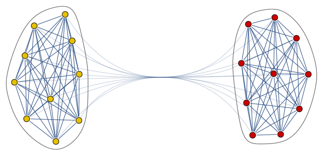
As written in the main article we can represent the interactions between the neurons in the body-clock as a network. In our case the network has two communities, where each community has many edges between the nodes, while there are only few edges between the nodes in different communities.
The network describes which neurons interact with each other, but it does not yet tell us how they respond to one another.
This is where the Kuramoto model comes in. The state of each neuron at each point in time can be thought of as the position of a dot on a circle, or equivalently as an angle between and . Here the subscript tells us which community the neuron is in (so for community or for community ), and the subscript tells us which neuron in that community it is, where we assume that there are neurons in each community, (so ). For the interaction we want that a neuron adjusts the time at which it fires as a result of some other neuron firing before it, either by firing a little earlier, or by firing a little later. The easiest way to do this is to adjust the neuron represented by angle as a response to the neuron represented by the angle via the sine of the difference between the angles, i.e., . Since a neuron is responding to all the neurons it is connected to simultaneously, it will adjust its angle by an amount that equals the sum of all the adjustments it would make for each neuron separately. In order to model the fact that the neurons are positioned in a fluid, we add a small random term to the total adjustment.
Kuramoto's model of synchrony
The Kuramoto model has been widely studied since it was conceived in 1975. Most studies have focused on the case where all angles interact with all other angles (i.e., the network is on the complete graph). Since this is clearly not reflecting the structure of the body-clock, we analyze what happens if we consider the Kuramoto model on a two-community network. For this purpose, we take the neurons in the same community to interact with a strength given by a parameter and the neurons in different communities to interact with a strength given by parameter , which can be positive, zero or negative. When is positive the two communities try to align with each other, when is zero there is no interaction and when is negative the two communities repel each other. We are interested in studying which states are possible for the system as a whole when we fix and and consider the number of neurons in each community to be very large.
What may we expect? In the Kuramoto model with the all-to-all interaction i.e., all neurons interact with all other neurons with strength , synchronization appears as a threshold phenomenon. This means that for values of below a critical value the neurons fire completely randomly, while for values of above the neurons start to fire in a synchronized way. When exceeds , synchronization is measured by what is called an order parameter. The order parameter for the synchronization is , which takes values between and , where represents the case where the neurons are completely unsynchronized and represents the case where the neurons are completely synchronized. We may therefore expect that synchronization in the two-community Kuramoto model will also appear as a threshold phenomenon.
If the environment in which the body-clock resides remains constant, then we may expect that the system will reach a stable and stationary synchronization level after some time. This means that the synchronization level will remain the same as long as the environment does not change.
Of course, in the two-community case we do not only want to know the level of synchronization in the body-clock, but also the synchronization in each community. In order to characterize all the possible stationary states, we also want to know the difference between the average angles in the two communities, which we call the phase difference and denote by . We found that the phase difference can only be or in the stationary state. In both of these cases, we can split the possible stationary solutions into three categories. In category (I) both communities are unsynchronized; in category (II) both communities are synchronized to the same degree (symmetrically synchronized); in category (III) both communities are synchronized, but one community is more synchronized than the other (nonsymmetrically synchronized).
The two-community version of the model has two parameters, and , which means that we do not have a single critical value, like in the one-community version, but have a critical line. The critical line, splitting the unsynchronized state (category (I)) from the symmetrically synchronized state (category (II)), is . The nonsymmetrically synchronized state (category (III)) is only possible in a part of the symmetrically synchronized section of the plane and requires when and when . The critical line dividing the symmetrically synchronized state and the nonsymmetrically synchronized state is identified as the solution to an equation involving special functions, which means that we cannot write down the solution explicitly. In order to visualize the situation, we plot the critical lines in Figure 1 below and indicate in which regions which solutions are possible.
Figure 1: In the light red region there is one pair of solutions: unsynchronized (U). In the light green region there are two pairs of solutions: unsynchronized and symmetric synchronized (S). In the light blue region there are three pairs of solutions: unsynchronized, symmetric synchronized and non-symmetric synchronized (NS). The left image is for the case and the right image is for the case .
Simulations
The previous section dealt with the possible stationary states. In the experiments with rats and mice one of the most interesting features that was observed was the possibility to see two different types of transitions to the phase-split state, which is certainly not something that can be understood by studying stationary states. In our model we did, however, see that stationary states exist in which the two communities have a phase difference of , which corresponds to the phase-split state observed in experiments. To study the transitions between these states (the one with and the one with ) is a mathematically intractable problem at the moment, but it is possible to see what sort of transitions are possible. The possible transitions that we observed are shown in Figures 2 and 3 below. Here, the average angle for community 1 and community 2 are given by and , and the synchronization levels are given by and .
Figure 2: Simulation of 10000 oscillators per community with (A) or (B) and . The time step is set at . The top images show the synchronization levels ( and ), the bottom images show the average phases ( and ). The phases are plotted in such a way that the different communities can be seen as the two components of activity in the suprachiasmatic nucleus. The time on the vertical axis can be regarded as consecutive days. (A) and (B) show the case where and are the same.
Figure 3: Simulation of 10000 oscillators per community with (C) and (D) and . The time step is set at . The top images show the synchronization levels ( and ), the bottom images show the average phases ( and ). The phases are plotted in such a way that the different communities can be seen as the two components of activity in the suprachiasmatic nucleus. The time on the vertical axis can be regarded as consecutive days. (C) and (D) show the case where and differ at first, but both approach 1 when the stable state is reached.
Interpretation
The simulations also show two different transitions between the symmetrically synchronized state with and the symmetrically synchronized state with , and back. In the first type of transition, both communities move to a higher level of synchrony together while their average phases either move further apart or move closer together. In the second type of transition, one community is forced to a much lower level of synchrony before it moves to the higher level of synchrony, while the other community moves directly to the higher level of synchrony. The first situation could possibly correspond to the smooth transition observed in the experiments, while the second transition could correspond to the chaotic transition.
There are two factors that seem to play a role in determining which transition occurs. The first is the initialization of the system and the second is the existence of the nonsymmetrically stationary state. When we start the simulation, we have to chose an initial state for the angles of the neurons. In experiments this state is difficult to interpret, but we can think of it as the situation that prevails immediately after a change of the environment in which the animals live has occurred (e.g. switch from light-dark cycle to constant light). The second factor is more easy to interpret: the strength of the interactions in the network is given by and , and if these are such that the nonsymmetrically synchronized state is possible, then the system might be forced to the nonsymmetrically synchronized state before it can move to the phase-split state.
Proceed to the Animation of the two-community Kuramoto model.
We want our guts to be filled with a diverse range of mutually beneficial and competitive interactions, a perfect blend of friends, frenemies, and enemies to keep our guts active and body on its toes. Read how networks can help understand these interactions!
During our teenage years, everything changes. It’s no surprise that our brain does too. But how do we make sense of this transformation? Is there a way to quantify it? Networks might just be the answer.
One of the main building blocks of modern AI-tools are artificial neural networks, abstract models inspired by the structure and functions of biological neural networks which enable machines to "learn". In this article, I will discuss some thoughts on this topic.
In this article, we will discuss a mathematical riddle that "seems impossible even if you know the answer". It is better known as the 100 prisoners problem.
If I give you a set of nodes, plus a way to find the distance between two nodes, how can you find all connections between these nodes as efficiently as possible?

 can be thought of as the position of a dot on a circle, or equivalently as an angle
  between
  and
and  . Here the subscript
  tells us which community the neuron is in (so
  for community
  or
or  for community
  ), and the subscript
  tells us which neuron in that community it is, where we assume that there are
  neurons in each community, (so
  ). For the interaction we want that a neuron adjusts the time at which it fires as a result of some other neuron firing before it, either by firing a little earlier, or by firing a little later. The easiest way to do this is to adjust the neuron represented by angle
  via the sine of the difference between the angles, i.e.,
  . Since a neuron is responding to all the neurons it is connected to simultaneously, it will adjust its angle by an amount that equals the sum of all the adjustments it would make for each neuron separately. In order to model the fact that the neurons are positioned in a fluid, we add a small random term to the total adjustment.
 and the neurons in different communities to interact with a strength given by parameter
  , which can be positive, zero or negative. When
  and
and  the neurons fire completely randomly, while for values of
  , which takes values between
  . We found that the phase difference
  in the stationary state. In both of these cases, we can split the possible stationary solutions into three categories. In category (I) both communities are unsynchronized; in category (II) both communities are synchronized to the same degree (symmetrically synchronized); in category (III) both communities are synchronized, but one community is more synchronized than the other (nonsymmetrically synchronized).
 . The nonsymmetrically synchronized state (category (III)) is only possible in a part of the symmetrically synchronized section of the plane and requires
  when
when  and
and  when
when  . The critical line dividing the symmetrically synchronized state and the nonsymmetrically synchronized state is identified as the solution to an equation involving special functions, which means that we cannot write down the solution explicitly. In order to visualize the situation, we plot the critical lines in Figure 1 below and indicate in which regions which solutions are possible.
 and the right image is for the case
  .
. and
and  , and the synchronization levels are given by
  and
and  .
.
 (A) or
  (B) and
  . The time step is set at
  . The top images show the synchronization levels (
 . The time step is set at