How to reconstruct a graph – The Network Pages

Imagine you want to send a letter to a friend across the country. After you put it in the mailbox, it seems to magically appear at their door. Of course this is not magic: it goes from your local post office, to a regional sorting center, then to another, and eventually to your friend's local post office before arriving. At each step, someone handles the letter and sends it on its way.

The internet works in a very similar way. When you send data from your computer - for example to load a webpage, stream a video or send a message - this data has to follow a certain route. It travels across a series of interconnected devices, called routers. Each router acts like a mini-post office, receiving your data packet and forwarding it to the next router on the path to its final destination.

To understand how the data travels over the internet, we can use TRACEROUTE. You give TRACEROUTE a destination, like google.com, and it then finds the entire journey your data takes to get there. It shows you every single router (a node) along the path, from your computer all the way to the destination.

But imagine that you don't want to know only how your letter travels to your friend, you want to know how all letters travel through the network. Then, instead of a single path, we will get millions of paths over millions of nodes. And every day, this network might change: making it very hard and time-intensive to find the complete network.

In this article we will have a look at the graph reconstruction problem. If I give you a set of nodes, how can you find all connections (edges) between these nodes as efficiently as possible? There are some rules: you only know that there are $n$ nodes in the graph, and you can only ask so-called 'queries' to me (or the 'graph oracle'): questions about properties of graph.

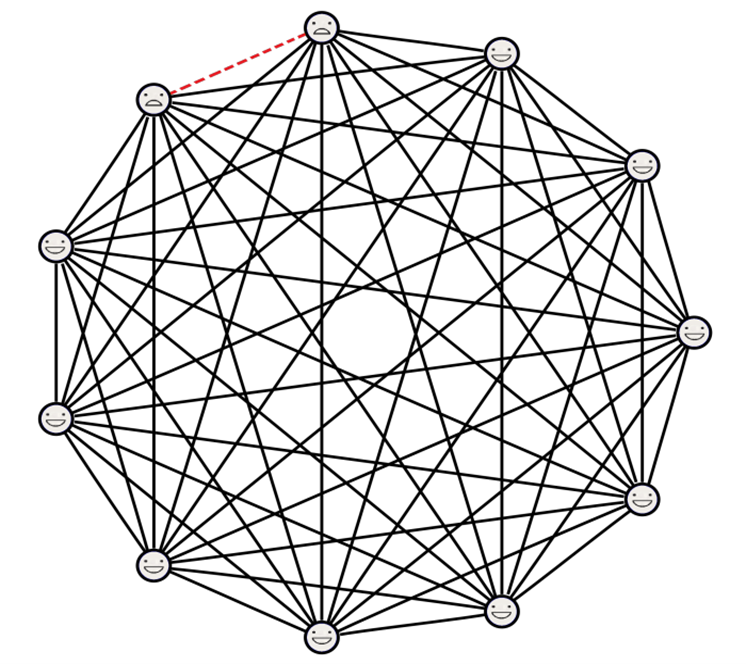
Today we are interested in shortest-path-distance queries. Suppose we have the following network:

If we ask a query about node $s$ and $e$ , we are given the distance of the shortest path between these two nodes, which we denote by $d(s, e)$ . This shortest path distance is the minimum number of edges we have to traverse to go from $s$ to $e$ . You can imagine this shortest path is very useful: this is also how we navigate the world. If want to know more about finding shortest paths, check out this article or this one!

Thus, in this case we have $d(s,e) = 3$ . This means there is no edge between $s$ and $e$ , since the shortest path from $s$ to e contains $3$ edges. If the distance between two nodes equals $1$ , however, there must be an edge between those nodes.

We want to find a strategy to find all edges in the graph with as little queries as possible. A simple upper bound on this number of queries is $n \times (n -1)$ : we perform a query for every node (of which there are $n$ ) with every other node (of which there are $n-1$ ), although we now count every node twice, so we can divide by 2. This totals $n(n-1)/2$ queries. For a network of 5 nodes, this means we have to do $(5 \times 4) /2 = 10$ queries, which is very doable. However, if we want to find all edges in an internet network with $10,000$ nodes, we would have to do $49,995,000$ queries. Suppose a query takes 1 second, then this means we would be querying more than 578 days!

Can we reduce this number of queries? Could, somehow, just a handful of queries be enough? No! In any case, we have to perform $m$ queries: one for each edge. This is because, as long as you do not query an edge, we cannot not know whether it exists or not.

So we have a theoretical lower bound ( $m$ queries), and an upper bound ( $n(n-1)/2$ queries). We want to find a smart way of finding all edges in a network, which is as close to the lower bound as possible. This means that the algorithm should query as few non-edges as possible. Let's first focus on general, bounded-degree graphs. Bounded degree graphs are graphs for which every node has at most $\Delta$ edges, where $\Delta$ is a constant (a fixed number). This is not important for now, but it is important if you want to prove the results that I will show you. Later, I will show an extension of the algorithm for geometric random graphs where every node has a location in space.

For general bounded degree graphs, Mathieu & Zhou proposed the SIMPLE algorithm¹. The general idea of this algorithm is to start with a complete graph with potential edges and eliminate all potential edges that cannot exist in the real graph. So, the algorithm goes from this graph:

To this graph:

We can eliminate these potential edges by doing queries. Let's look at the example graph above. We focus on nodes $s, a$ and $e$ in the figure. Suppose that we know the following:

$d(a, s) = 1$ , and
$d(e, s) = 3.$

From these two queries, we can deduce three things:

There is an edge between node $a$ and node $s$ ,
There is no edge between node $e$ and node $s$ , and
There is no edge between node $a$ and node $e$ .

The first two observations follow directly from the two queries: a shortest path query of $1$ tells us there is an edge and a shortest path query of $3$ tells us there is no edge. This last observation follows from the two queries together. Suppose there is an edge between node $a$ and node $e$ . Then we could go from $s$ , to $a$ , to $e$ using only two edges. So $d(e,s)=2.$ This is not possible, because the query tells us that $d(e,s)=3$ . Therefore, there cannot be an edge between node $a$ and node $e$ .

Thus, we have confirmed one potential edge and eliminated two! The state of our algorithm at this point is:

Here, red means an edge has been eliminated (it cannot exist) and green means the edge exists.

Now, let's generalize this observation: we can eliminate all potential edges between nodes $v$ and $w$ for which \begin{equation} |d(v, s) - d(w, s)| > 1. \end{equation} In other words: we can eliminate all potential edges if the difference between their shortest paths to some node $s$ is larger than 1.

After these two queries, let's do two more queries:

$d(b, s) = 2$ , and
$d(c, s) = 2$ .

Since the shortest path from b to s and from c to s is larger than 1, we again can eliminate both potential
edges.

Now, there are only 4 potential edges left, which we will query directly. In total, we have done the following 8 queries to obtain the full graph:

$d(a, s) = 1$ ,
$d(e, s) = 3$ ,
$d(b, s) = 2$ ,
$d(c, s) = 2$ ,
$d(a, c) = 1$ ,
$d(a, b) = 1$ ,
$d(e, b) = 2$ ,
$d(e, c) = 1$ .

In total, we performed $8$ queries for this graph of $5$ nodes. Now you may notice that we start querying distances to $s$ . Why did we choose a 'special' vertex $s$ ? In the SIMPLE algorithm, we choose approximately $\log(n)$ of these nodes $s$ and call this the seed set $S$ . This seed set is just a random subset of all the nodes in the graph. We call these seeds as we start with these nodes and do a query with these seeds against all other nodes in the graph. This gives us a starting point to eliminate edges. ²

Let's discuss the full SIMPLE algorithm. This algorithm works as follows. We start with a subset $S$ of all nodes: the seed set. We also define the set of all potential edges $E$ , which initially consists of all node pairs $\{a, b\}$ for all distinct $a, b \in V$ .

For every seed $s \in S$ and node $a \in V$ , query $d(s,a)$
- If $|d(s, a) - d(s,b)| > 1$ , there is no edge between node $a$ and $b$ . We remove $\{a,b\}$ from the set of potential edges $E$ .
For all potential edges $\{a, b\}$ in $E$ , query $d(a,b)$ .

After step 2, we are done and we found all edges! We start with querying all nodes with a small set of nodes. If this is not too large, it only costs us $|S| \times n$ queries. Then, in step 2 of the algorithm we still do $|E|$ queries extra, to check all potential edges that we did not eliminate yet.

The proof that this set $|E|$ is small is not easy, so I will skip that here. The authors of the SIMPLE algorithm show that this algorithm can find all edges in a graph with $O(\log(n) n^{5/3})$ queries, and that it works for all general, bounded-degree graphs.

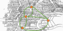
When me and my colleague heard of this algorithm, we were wondering whether it could work even better for special types of graphs. In specific, we checked out geometric random graphs, where nodes have a position and edges only exist between nodes that are a distance less than $r$ apart. Almost every real-world network has an underlying geometry: the internet network routers are located in the world; in a social network, your friends often live close to where you live and a train network connects cities that are close to each other.

Our idea was that this should allow for faster reconstruction as you have more knowledge on the edges: there will not be edges between nodes that are far apart.

An example of a geometric graph

We found out that this geometry indeed causes a faster reconstruction time! We can decrease the number of queries because we can eliminate even more potential edges in the geometric graph, because we know that edges can only exist if the distance between two nodes is less than $r$ .

To prove this (or at least give some intuition), we have to introduce another distance. We already discussed the shortest path distance, but we now also use the Euclidean distance, which we denote by $d_E(a, b)$ . The Euclidean distance is the straight-line distance between two points - also called `as the crow flies'. If you could fly directly to a location in a straight line, without following roads or paths, the length of that line is the Euclidean distance.

If we know that the shortest path distance $d(a,b) = 5$ , we know because of the geometric graph that these nodes have an Euclidean distance of at most $5 r$ apart in Euclidean distance. Dani et al.³ also found a lower bound: if $d(a,b) = t$ then $d_E(a,b) \geq \frac{r(t r^{4/3}-c \log(n))}{c + r^{4/3}}$ .

Using these bounds, we can then find an approximate location of every node after we did some querying. This means that we can eliminate even more potential edges, as we know that nodes that are far apart will not have an edge. Therefore, there are relatively few potential edges, as those can only happen locally. And that is why we can efficiently reconstruct geometric random graphs!

If you want to know more about Lotte's research, click here.

In the paper, we consider geometric random grapsh with $n$ nodes and let $n$ go to infinity. Moreover, we look at two regimes: the dense and sparse* regime. In the dense regime, the graph has connection distance $r = n^k$ , $k \in (0, 1/2)$ , which means that there are many edges. In the sparse regime, the connection distance $r \geq \sqrt{\log(n)}$ , so the graph has less edges (but is still connected).

For dense graphs, we can reconstruct the graph in $O(\log(n) n^{3/2-4k/3})$ queries if $0 < k < 3/20$ and $$O(\log(n)n^{2k+1})$ queries if $3/20 \leq k < 1/2$ . This latter bound does seem very large, but is almost optimal: there are many edges ( $O(n^{2k+1})$ ) since every node connects to all edges within radius $r = n^k$ . And, as we said before, we should query at least all edges at least once. Therefore, our result is, up to a log-term, optimal!

For sparse graphs, the full reconstruction can be done in $O(\log(n)n^{3/2})$ queries.

Both regimes show an improvement for the bound of the SIMPLE algorithm, which is $O(\log(n)n^{5/3})$ .

*but not fully sparse, it still has to be connected!

Mathieu, Claire, and Hang Zhou. "A simple algorithm for graph reconstruction." Random Structures & Algorithms 63.2 (2023): 512-532.\\ ↩︎
By using simulations, I found out that in the geometric random graph, only 4 seeds - one in every corner - is enough to reconstruct the entire graph very efficiently! This works because these 4 strategically chosen seeds maximize the number of potential edges we can already eliminate because the difference in graph distance to two nodes is larger than 1. ↩︎
Dani, Varsha, et al. "Reconstruction of random geometric graphs: Breaking the $\Omega(r)$ distortion barrier." European Journal of Combinatorics 121 (2024): 103842. ↩︎