Twenty years ago, driving to your holiday destination was a tedious task. You had to plot a route in a paper road atlas and keep track of where you were on the map. After a wrong turn, the holiday spirit would be spoiled by a fight in the car: was it the driver's fault, or the navigator's?
Nowadays we have route planners such as TomTom and Google Maps to make driving to a holiday destination a lot simpler. Using your GPS location and your target address, they compute an optimal route in the road network and show you in real-time which directions to take. (And if anything goes wrong, you can just blame the machine!) In this article we explain the science behind these route planners. In 1959, the Dutch mathematician and computer scientist Edsger Wybe Dijkstra invented an algorithm for finding shortest paths in a network, which is still one of the best algorithms today. It has become known as Dijkstra’s algorithm and is taught to computer science students all over the world. This article will show you how it works.
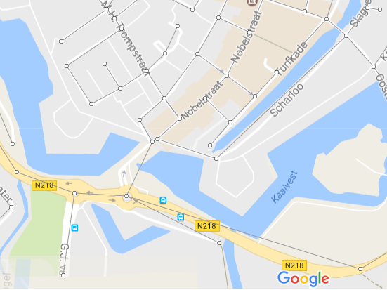
Below you see part of the road network around Brielle, a beautiful town in the west of the Netherlands. The drawing simultaneously shows the road network like you would see it on Google maps, together with the mathematical representation as a graph consisting of vertices (circles, representing intersections) and edges (black lines, representing road segments). Notice that a real-life road on the network is often split into multiple edges: each edge represents a part of the road between two consecutive intersections. To be able to do its job, the road planner stores this graph in its memory. For each edge, it also stores the length of the corresponding road segment in meters.
To see the algorithm in action, click on a location in the figure below. The algorithm will then start its computation on the graph, using your chosen location as the starting point of the journey. You can control the speed of the animation using the slider.
Before explaining which steps the algorithm takes, let's have a look at what the outcome of the algorithm is. When the algorithm has finished, it has highlighted a part of the network in red, and it has chosen a direction for every red edge. Everything you might want to know about shortest paths in this network is encoded in the red highlighted network! At first, this may appear strange: how can the algorithm already be done when you have only told it where your journey starts, and not where it ends? The answer is simple: the algorithm has simultaneously found a shortest path to every potential destination in the graph!
To see what this means, hover your mouse over the vertex of your desired destination in the graph. The drawing will then highlight a shortest path from the chosen starting point, to this destination. Notice that this path is formed in a very simple way: the path is determined by repeatedly following red edges in the direction of the arrow, until arriving at the starting point. Driving along this path in the opposite direction then gives a quickest way to reach your destination! So the highlighted edges, together with their orientation, represent shortest paths to any potential destination in the graph. That's why this outcome of Dijkstra's algorithm gives your route planner everything it needs to guide you to your holiday address.
Now that we have seen how the algorithm operates on a large road network, we have a detailed look at a small example to explain exactly what it does. The drawing of the graph below shows the structure of the example network, as well as the length of each edge. For example, the horizontal edge at the top represents a road segment of 6 meters in length. Click on the 'Show once more' button in the drawing below to (re)start the animation.
The close-up view shows Dijkstra's algorithm running on the small graph, where the starting point of the journey is the left-most vertex. For each vertex of the graph, the algorithm keeps track of the shortest path to that vertex it has discovered so far. The total length of the current-best path is drawn as the label of the vertex. When the algorithm starts, it knows that you can get from the starting point to the starting point by a path of 0 meters (because you're already there!). For vertices to which no path has been discovered yet, the label is ∞, the mathematical symbol for infinity. When the algorithm is done, the label of each vertex is equal to the total length of a shortest path to that vertex, starting at the very left. For example, the label of the rightmost vertex is 5 when the algorithm finishes: the corresponding shortest path consists of three edges: two of 2 meters, and one of 1 meter.
Dijkstra's algorithm works by repeatedly selecting a vertex and using that vertex to discover new paths. In the animation, the vertices that have already been selected in the past are grey, the vertex that is currently active is yellow, and the remaining vertices are white. In each round, the algorithm selects the vertex with the smallest label that has never been selected before (a white vertex). Let’s call this the active vertex. In the first round, the algorithm always selects the starting point as active vertex because it has label 0.
Suppose that a vertex is made active that has a label value of L, for example L=3. Since the label of a vertex represents the length of a shortest path to that vertex that has been discovered so far, the algorithm already knows a path from the starting point to the active vertex of L meters. If the graph contains an edge that connects the active vertex to a neighboring vertex (in green), then that edge together with the path to the active vertex, forms a path from the starting point to the neighbor. If the edge has a length of X, then this newly discovered path has length L + X. If L + X is smaller than the label of the neighbor, then the algorithm has discovered a new path to the neighbor that is shorter than all paths it knew before! It then does the following:
it changes the label of the neighbor to L + X, the length of the newly discovered path, and
it adds an arrow from the neighbor to the active vertex, to show that the best path goes via the active vertex.
If there was a previous arrow leading out of the neighbor, this arrow is removed because a better path has been discovered. After updating the labels of all the neighbors of the active vertex, the algorithm is done with it, makes it gray, and selects a next active vertex. When all vertices have been selected once, the algorithm is done! Dijkstra proved mathematically that when the algorithm has finished, following the arrows gives the shortest paths in the network.
Now that you’ve learned what the algorithm does, why don’t you look at the animation again to see if you can understand what is happening? Can you explain:
why the algorithm selects the top-left vertex as the active vertex in the second round?
why the label of the top-right vertex changes from ∞ to 1+6=7 in the second round?
why the label of the top-right vertex later changes from 7 to 2+2=4 in the third round?
If you can answer all these questions, then you have mastered Dijkstra's algorithm. Every individual step that the algorithm takes is very simple; you could easily do it on a piece of paper by hand. But since road networks are very large - the road network of Western Europe has more than 18 million vertices! - it’s nice that we have computers to do this job for us.
During our teenage years, everything changes. It’s no surprise that our brain does too. But how do we make sense of this transformation? Is there a way to quantify it? Networks might just be the answer.
Elisabeth already has an idea in mind: she would like to find the fastest possible route that goes to each address exactly once before finally returning to the station. This task is a well-known mathematical problem, namely the Traveling Salesman Problem (TSP)! How can she solve it?
Getting to class on time isn't hard, if you leave on time and know the fastest route. But what’s the fastest route when the hallways are crowded? For their final high school project, Dylan and Tobias worked on finding the most efficient ways to navigate school during peak hours.
If, after reading the title, your immediate response is to shout "1/6-th", then you have correctly answered the question. Well done! However, in this article we will focus on the meaning of this question. What exactly is this "chance" of which you've just exclaimed it equals 1/6-th?
If I give you a set of nodes, plus a way to find the distance between two nodes, how can you find all connections between these nodes as efficiently as possible?