Imagine you’re in a remote village and only have a limited number of vaccines to distribute to protect the community from a deadly virus, who do you vaccinate?
A difficult decision, but necessary. Assuming that the disease is just as deadly for everyone in the community, the best way to prevent deaths is to contain the spread of the virus. But which are the most important members of the community to protect to minimise the spread of the virus? This quickly becomes a philosophical question, where there is no clear right or wrong answer. And while this might be interesting from a philosophical point of view, we can't do much with this dilemma in mathematics. However, we do have a clear goal, namely minimising the spread. And with this in mind, we can rephrase the question into one we can solve using mathematics. To do this we have to give a mathematical meaning to the words important and protecting.
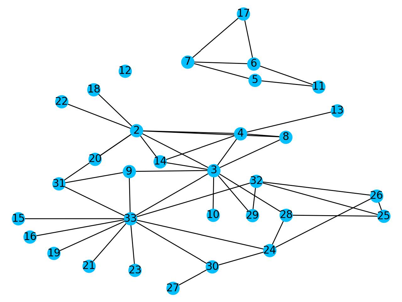
To know how the disease spreads we first need to map out who is in contact with whom. We can do this using a network. Networks are represented in mathematics using graphs, which are collections of points, called nodes, which are connected by lines, which we call edges. In the situation described above, the nodes are different members of the community, and the lines between them stand for contacts where transmission of the virus is possible. In this model to "protect" a node means to remove it from the network. In the real world, removing a node can be seen as vaccinating someone.
This does, however, directly bring uncertainty into our model. Human behaviour is complex and difficult to perfectly register. Furthermore, there can be a large grey area in how close contact has to be for transmission to be possible. Thus, especially for larger populations, it often isn't possible to determine the social network explicitly. In these cases, other methods from a modern branch of mathematics called network science are available to create a network that captures the main structure of the underlying social network.
The power of eigenvalues
The virus can only spread from one node to another node if there is an edge connecting the two. Of course, we could look at the network to see which nodes are connected, but we can't perform calculations with just the network. To perform the necessary calculations we move up one level of abstraction by representing the connections between nodes in a matrix. This is useful because in mathematics we have developed an extensive toolbox to work with matrices.
This is where an adjacency matrix comes in. This is a matrix where the rows and columns stand for the nodes and an element in the matrix gets awarded a 1 if there is an edge between the two nodes indicated by the place in the matrix and a zero if there is no connection. For an example see the figure below.
Figure: On the left we have the adjacency matrix belonging to the graph on the right.
One of the reasons we like to work with matrices is that we can summarise many of the important qualities of a matrix into a couple of numbers, namely the eigenvalues. Remember that an eigenvalue is a number such that there exist a vector , called and eigenvector, such that . The reason why we can look at eigenvalues instead of the whole matrix is that if two matrices have the same set of eigenvalues, then they are for all intends and purposes the same matrix. This is because we can always rewrite one matrix in terms of the other. For a more in-depth reminder of what eigenvalues are, see this video from 3Blue1Brown.
Translating intuition into a formula
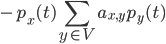
So we've now increased our toolbox to describe our network with the adjacency matrix and its eigenvalues. Let's go back to the village and the situation at the beginning of the article. We consider the case that people can be either susceptible or infected, people who get infected recover and become susceptible again. This may seem restrictive at the moment but later we will see that the main result we describe holds in more general cases as well. The goal is to prevent the spread of the virus, given we know the network of contacts between people. To do this we need to describe how the probability of a node being infected changes in a small time step . To derive an equation for this probability we need to know two things, namely, how long it takes to recover after being infected and how likely it is to get infected after a contact with an infected node. We say that the rate at which nodes recover after infection is equal to some value , and the rate at which susceptible nodes get infected is equal to some value . This is given by the following equation:
There are two possibilities for each node; it can either be infected or susceptible. The probability that a node will be infected at time is the chance that it was infected at time plus the chance that the node changes states. A node can either go from infected to susceptible, or the other way around. The probability for the first scenario, i.e. that a node goes from infected to susceptible, is the chance that a node was infected at time , times the chance of recovery in a time step , given by . For the second scenario, we need to multiply the chance of the node being susceptible at time and getting infected. The chance of getting infected is a sum of the chance of getting infected by a specific node , under the condition that there is an edge between and . This is given by the term. Putting this all together gives the equation above.
We can rewrite this equation into a differential equation:
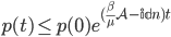
Sadly this isn't a differential equation for which we know the exact solution. We can however give an upper bound for the solution by removing the term. To simplify the equation a bit more we map to . This gives us
This differential equation does have an exact solution, namely . The main thing to take away from this solution is that the chance of a node getting infected is an exponential function. Thus if what is raised to the power of is small enough the number of infected nodes will decrease exponentially. Here is where eigenvalues come and do their magic! The size of is related to the largest eigenvalue , so if , then will go to zero exponentially.
The intuition behind this is that most of the important qualities of a matrix are captured in the eigenvalues. Let's take now a moment to reflect on something we mentioned before. We supposed that nodes become susceptible again after recovering from an infection. In reality, it may happen that nodes that recover become immune. In such a situation the equation we derived above needs to be adapted, but the upper bound we have derived is still correct! The main result thus holds in more general situations that the one discussed here in detail.
Requirements to protect the network
We thus find that if the largest eigenvalue is smaller than , then over time the number of infected nodes will go to zero. The term tells us something about the rate of recovery over the rate of infection. It is intuitive that if a node is more likely to go from the infected state to the recovered state than the other way around that then the infection will die out eventually. So if is small then the infection doesn't want to die out naturally. We can't in most cases change since these parameters are given by the real-world problem we're trying to solve. Instead we thus need to reduce by removing nodes from the network in order to get , we call this a reduction in a drop in eigenvalue.
Finally, we've arrived at a mathematically rigorous way to pose the question we started with. Thus instead of asking: what are the most important nodes in the network to protect?, we have rephrased the problem into: what nodes will result in the largest drop in the largest eigenvalue when removed from the network?. With this question, we can now return to our remote community and figure out the best way to distribute the vaccines.
We can however go even further. Since we've developed an abstract mathematical model we can now solve a wide array of problems. We can namely apply the previous steps to other problems that also have an underlying network and something that spreads through the network. For example, if a dangerous bacteria is discovered in a water treatment plant. We have a filter to remove the bacteria from a basin and prevent the spread to other basins. However, you don't have enough filters to protect all of the basins. Or imagine you're responsible for safeguarding a computer network of a company from computer viruses and you want to know what the most important computers and hard drives are to protect in the network to prevent as many links in the network when a computer gets infected. Finally, let's look at the electricity grid of a country. If one power distribution centre for instance gets overloaded and goes dark it puts more strain on the nearby centres, which might cause them to go dark as well. You have a limited amount of money at your disposal to fortify a couple of power distribution centres to best prevent blackouts.
All these problems seek to answer the following question: what are the most important points in my network to protect?. So, we can again rephrase this question into: what nodes will result in the largest drop in the largest eigenvalue when removed from the network?. The only thing that changes between the different applications is what a node and edge stand for, and what spreads in the network. But with the abstract model we have constructed, this doesn't change anything. This is exactly what makes a more abstract model so powerful. It is important to note at this point that the largest eigenvalue is not the only number of a network that yields information on how an epidemic spreads on a network. Researchers have proposed other numbers as well which can be used, one example being the largest degree.
A virus in a karate-club
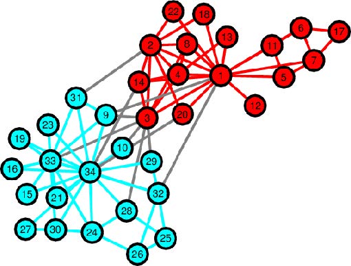
To see the effect of removing a node on the largest eigenvalue we can look at the example of the karate club network. This is a network based on a university karate club in 1977. Here each node represents a member of the club and an edge represents close contact between two members of the club. The largest eigenvalue that belongs to this graph is around 6.73. Now we look at two scenarios, you can remove one or two nodes from the network. Now for more realistic networks, which are much larger, we need special algorithms to give us the nodes which result in the largest eigenvalue drop. But for this small network, we can figure it out by looking carefully at the network.
The graph of the karate club network, where the two colours stand for the two groups in which the club split when an argument broke out between node 34 and 1.
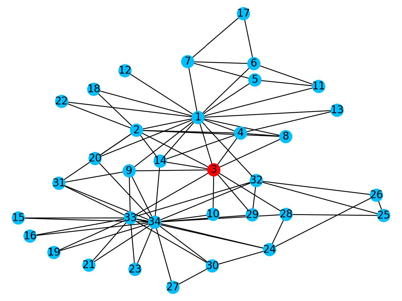
For one node removing node 3 will give us the largest eigenvalue drop, where we go from 6.73 to 6.09. The intuition behind this is that node 3 is the node that connects the red and blue areas of the network together. So if we remove this node we automatically protect half of our network. Hence we see that the best node to remove from the network may not be necessarily the node with the highest degree.
We want to remove node 3, since this gives the largest drop in eigenvalue.
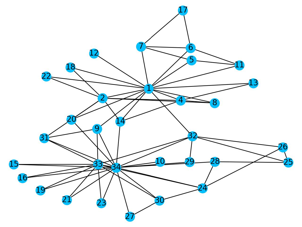
After removing node 3 we're left with this network.
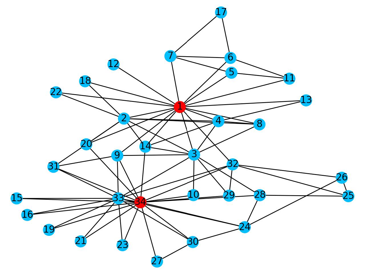
If we're able to remove two nodes the nodes that will result in the largest drop in eigenvalue are nodes 1 and 34, where we go from 6.73 to 4.62. We see that these are the two nodes at the centre of the blue and red sections respectively. So removing these nodes halts the spread within a section the most.
If we can remove two nodes from the network we want to remove nodes 1 and 34.
After removing node 1 and 34 we're left with this network.
For an average social network, the graph is way too large to be able to find the nodes which results in the largest drop in eigenvalue by hand. Just visualising a network of all social contacts in Amsterdam is difficult enough, let alone identifying the nodes that result in the largest drop in the maximal eigenvalue. For this algorithms have been created, like the NetShield algorithm for example, and a lot of work is being done on improving these algorithms.
Although it took some work to get here, we now have a well-formulated and concrete problem that we can solve using mathematics. This means that if we are faced with a new real-world problem we don't have to solve it from scratch, but we can instead check a couple of conditions or check whether certain assumptions are reasonable and if that is the case we have a way of getting a solution ready-made.
This article was inspired by a lecture on this topic given by Luca Avena from Leiden University.
If, after reading the title, your immediate response is to shout "1/6-th", then you have correctly answered the question. Well done! However, in this article we will focus on the meaning of this question. What exactly is this "chance" of which you've just exclaimed it equals 1/6-th?
During our teenage years, everything changes. It’s no surprise that our brain does too. But how do we make sense of this transformation? Is there a way to quantify it? Networks might just be the answer.
We want our guts to be filled with a diverse range of mutually beneficial and competitive interactions, a perfect blend of friends, frenemies, and enemies to keep our guts active and body on its toes. Read how networks can help understand these interactions!

 important
 and
and  comes in. This is a matrix where the rows and columns stand for the nodes and an element in the matrix gets awarded a 1 if there is an edge between the two nodes indicated by the place in the matrix and a zero if there is no connection. For an example see the figure below.
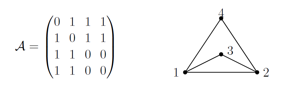
 is a number such that there exist a vector
  , called and eigenvector, such that
  . The reason why we can look at eigenvalues instead of the whole matrix is that if two matrices have the same set of eigenvalues, then they are for all intends and purposes the same matrix. This is because we can always rewrite one matrix in terms of the other. For a more in-depth reminder of what eigenvalues are, see this video from 3Blue1Brown.
  being infected changes in a small time step
  . To derive an equation for this probability we need to know two things, namely, how long it takes to recover after being infected and how likely it is to get infected after a contact with an infected node. We say that the rate at which nodes recover after infection is equal to some value
  , and the rate at which susceptible nodes get infected is equal to some value
  . This is given by the following equation:
 is the chance that it was infected at time
  plus the chance that the node changes states. A node can either go from infected to susceptible, or the other way around. The probability for the first scenario, i.e. that a node goes from infected to susceptible, is the chance that a node was infected at time
  . For the second scenario, we need to multiply the chance of the node being susceptible at time
  , under the condition that there is an edge between
 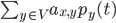 term. Putting this all together gives the equation above.
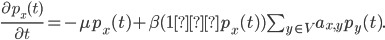
 term. To simplify the equation a bit more we map
  . This gives us
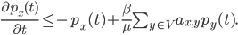
 . The main thing to take away from this solution is that the chance of a node getting infected is an exponential function. Thus if what is raised to the power of
  is small enough the number of infected nodes will decrease exponentially. Here is where eigenvalues come and do their magic! The size of
  , so if
 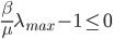 , then
  will go to zero exponentially.
 , then over time the number of infected nodes will go to zero. The
  is small then the infection doesn't
  , we call this a reduction in