The results of supposedly perfect and accurate machine learning models can be deceived by slight perturbations in the data. Let's see how! Maybe you have seen this funny scene from The Mitchells vs. the Machines where two robots fail to recognize Monchi as a dog.
Of course we are not there yet where robots will be walking among us, but the confusion described in the video may not be too far from reality. Lets see what happens in reality nowadays.
Applications of machine learning models are everywhere, with many online platforms and major science fields using tools relying on machine learning. Take, for example, image recognition and computer vision. Many real-life applications of vision systems include autonomous vehicles, facial recognition, medical imaging, classification of objects, and whatnot. These models are trained to be precise in taking data-driven decisions even when the data is complex. Training, in this context, refers to using historical data to analyse and identify specific patterns or behaviour. So, to begin with, what kind of models are we talking about?
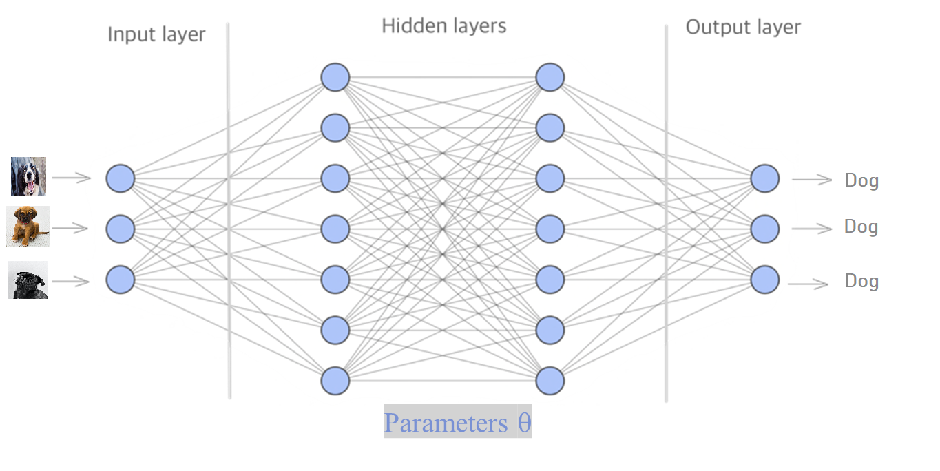
In simple terms, they can be described as mathematical equations relating input values to some output. Such models often depend on parameters (weights) that transform the input into the output. For instance, in image recognition, the input can be images of animals, and the output is "Dog" if the animal in the picture is a dog, and "Not a dog" otherwise. The field of machine learning relies heavily on mathematical equations and networks to create algorithms that can "learn". Artificial neural networks are a particularly popular and widely used mathematical model of machine learning.
Models inspired by our neurons
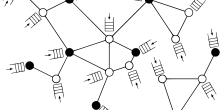
A neural network architecture consists of one input and one output layer, and several hidden layers. All these layers contain nodes and connections between the nodes, creating a network. The input is given to the input layer. Afterwards, it is forwarded to the nodes in the hidden layers following the connections of the network. In the hidden layers the input is transformed, and the computed values are forwarded to the output layer. At each node in the hidden layer, a mathematical equation transforms the value that was forwarded to it from the previous layer, and forwards its output to the nodes in the next layers.
All the mathematical equations in the hidden layer depend on parameters, which we will just denote by . For the purposes of this article we don't need to know exactly what these are. The question is now, how can we tune the values of all these parameters so that the neural network makes correct predictions? Meaning, that given a random image of an animal, it can correctly classify if the animal is a dog or not.
To achieve this we "train" the network. To train a neural network we need a dataset consisting of combinations of input values and output values. For each input value in this dataset, you will first let the network compute its own output value. In the next step, we compare this computed value with the correct output value, and tell to the network how far it is from the correct output value. Afterwards, we update the parameters of the equations in the nodes of the network to get closer to the actual output. By training the neural network with sufficiently many data we hope that the parameters are improved in such a way that the network can give correct outputs also for new input values that were not in the dataset used to train the network. This whole concept of training a neural network can be described with mathematical precision, lets see how!
The math behind training the network
The concept of training a neural network corresponds to applying some mathematical functions on the input data in the hidden layers. In this article, we discuss in detail so called linear-models, and we will show that these models can be easily tricked to give totally weird results, as in the video with Monchi! Let's start with a simple example, of a single node in each layer, the input, output and hidden layer.
In the node in the hidden layer we just apply a linear function to the input value and forward the output to the output layer, hence if the input is the output will be
for some values of the parameters and . To construct a more advanced neural network which will be able to perform beter we add more nodes, connections and hidden layers, like in the image below.
To construct a more advanced neural network which will be able to perform beter we add more nodes, connections and hidden layers.
In this case, the equation transforming the input into the output is more advanced but can be still linear, in this case at each node in the hidden layers a linear equation is applied to the input from the previous nodes, and the output is forwarded to the next nodes following the connections of the network. The mathematical transformation you will apply to the input at each node can be chosen differently, you could also choose a quadratic function, or a sigmoid function.
The art in constructing neural networks that work properly lies into choosing these mathematical functions which will transform the input to the output, and also choosing how many hidden layers and nodes will be used in the network. This is a delicate step, because too few layers can lead to a network that performes poorly (underfitting), but too many layers can lead to a network that is too specialized (overfitting) to properly predict the output of a new input that was not in the dataset used to train it.
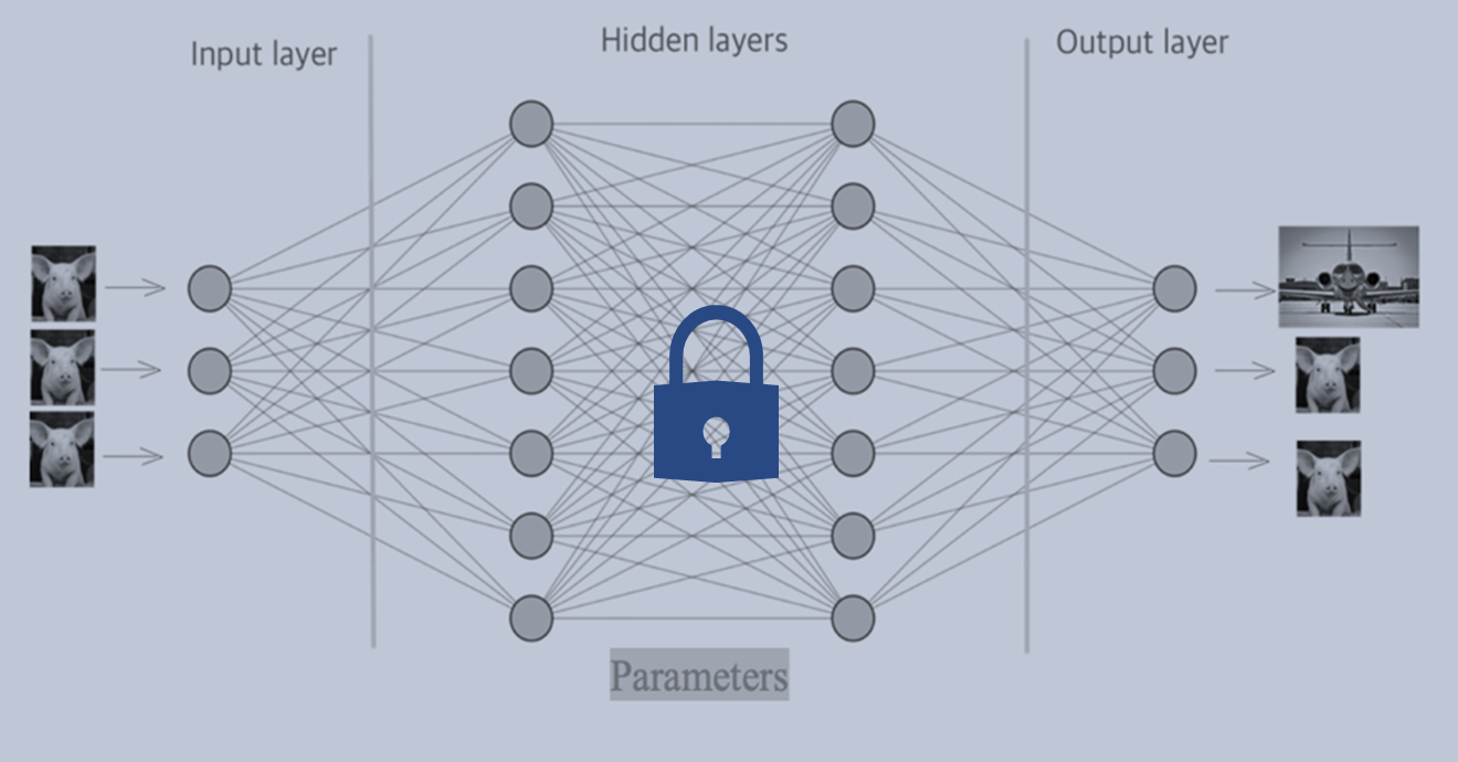
Suppose we have managed to construct a neural network that seems to perform pretty well. Whenever the input is an image of a dog it gives as output "Dog", whenever it is a pig it gives as output "Pig", and whenever something else it gives "Not a dog or a pig". We are happy and we can start using the neural network. Unfortunately, the neural network may still have some weak spots, that malicious adversaries may use to mess up with the predictions it make. It is important to have a good understanding of such weaknesses of the neural network. Do you, for example, see any difference in the following two images?
I am pretty sure that it is not possible to spot any difference with a human eye, but amazingly the (linear) neural network constructed above may misclassify the second image as an "airplane"! Crazy right? Well, if you write down the mathematics you will see it is not so crazy, a careful analysis shows why this happens! Bare in mind, that for the neural network an image is just a huge collection of pixels, each one with some characteristics, like its color. Let's see how an adversary can create such confusion to the neural network.
Attacking the network
This confusion can be created to the network by adding very small noise in the image which is not visible to human eye, which will very likely lead to a strong misclassification.
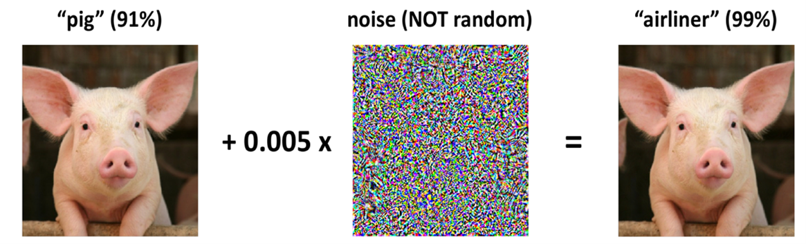
The following figure is one of the most classic examples, where the left image is correctly classified as “pig” by the network, but when a slight noise of 0.005 is added, and given as input to the trained classifier recognises this image is classified in 99% of the times as “airliner”. In the literatuur this is called pixel attack. There are also results showing that changing even only one pixel can lead to misclassification. Such misclassification are not just limited to 2D but also 3D objects.
Figure 1: Adversarial example with noise constraint of on ImageNet (Deng et al., 2009) dataset. The left image is the original, and the right image is the original plus the noise image shown in the middle.
Such a malicious action of adding some weird noise into images just to mess up with the neural network we have constructed, is an example of an adversary attack. Moreover, what’s surprising is that how only “linearity” of these models can also be a cause for the generation of such confusion. Let’s try to understand in a nutshell how this happens.
Say instead of input we give the perturbed input is ( in the picture above) to the network, for some sufficiently small. Conventionally, it is anticipated for the classifier to place both and in the same class if is very small but, surprise surprise!! That’s not the case anymore. Considering the products between the parameters at node and an adversarial input we get that node will give as output:
We can see that the perturbation at node here grows by . Although this mistake may seem small for each node, we have to see what happens when alls these small mistakes, in all the nodes in a layer, are combined with each other in the output. Suppose that the parameters have magnitude equal to , and that there are nodes in the layer. Then the total error will be increase by ! Which can get very large if and are large! Hence a very small perturbation in the input, which cannot be seen with a human eye, can lead to a wrong classification in some cases.
In general, adversarial attacks on machine learning models, such as artificial neural networks, rely on the manipulation of input data in a way that causes the model to make incorrect predictions. One of the key mathematical concepts behind these attacks is the concept of gradients. A gradient is a vector that points in the direction of the steepest increase in the output of a function, such as the output of a neural network. Mathematically, the gradient of a function with respect to is represented as . By calculating the gradient of the output of a neural network with respect to its input, an attacker can find the direction in which small changes to the input will cause the greatest change in the output. This is known as the gradient descent method.
Types of Adversarial attacks
There are two different kind of attacks. We have white-box (as the perturbation discussed above) and black-box attacks. The type of an attack depends on whether the attacker knows the target’s machine learning-model and its parameters, or has no access to the model, but only to its output.
In white box attacks, the attacker has full knowledge of the target model, including the architecture, the parameters, and the training data. These types of attacks are typically easier to execute because the attacker can use this knowledge to create more effective adversarial examples. Attackers are fully aware of the weak spots of the machine learning model used and can target them easily.
In black box attacks, the attacker has no knowledge about the internal workings of the target model and can only interact with it through the input and output interface. These types of attacks are often based on the concept of transferability, which is the idea that adversarial examples found on one model can also be used to attack other models. For example, an attacker could use an adversarial image that was created to fool a model trained on dataset A, and use it to fool a different model that was trained on dataset B. Now that we know how adversarial attacks can be performed it’s time to understand what can be done to prevent them.
The idea revolves around generating a lot of adversarial examples and adding them to the dataset we will use to train the network. In this case, the network will be trained to classify both images, with or without white noise, correctly. Hence we train the neural network not only to do the classification, but also not to be mislead by adversarial attacks. This strategy is called adversarial training.
However, in reality, there are more chances of black-box attacks for which there are two strategies to attack. The first one being transferability across algorithms, where attackers additionally have no knowledge of the training algorithm used, i.e. only the inputs and outputs are known. The second being referred as transferability across policies where, the attackers have access to the training environment and also have knowledge of the training algorithm. They know the neural network architecture of the target policy network, but not its random initialization i.e. the initial values given to parameters.
Hence we train the neural network not only to do the classification, but also not to be mislead by adversarial attacks. This strategy is called adversarial training.
Ensemble Adversarial Training is the best proposed algorithm as of now to prevent black-box attacks. In this kind of training, the dataset is enriched with samples generated from other neural network models. In this way, the network is trained to classify properly and will be protected from adversarial attacks trying to confuse the network and fool it into making wrong predictions.
Understanding adversarial examples is not only important for defending against attacks on machine learning models, but also for designing more robust and secure models. By gaining knowledge on the mathematics behind these attacks and the types of attacks, we can develop better techniques to identify and prevent them. Additionally, this knowledge can aid in the development of more secure and reliable AI systems that can be used in real-world applications.
As we move forward with the integration of machine learning in our daily lives, it is vital to be aware of the potential risks and limitations of these models. To do so, we can ask ourselves questions such as: "How can we design models that are more robust against adversarial examples?" or "What are the real-world implications of adversarial examples on AI-powered systems and how can we mitigate them?". These questions will help us to continue to push the boundaries of what is possible with machine learning and AI, while ensuring that we do so in a safe and responsible manner.
This is a question I have been thinking about for the last two years. In this article, I will give a little overview of what I have discovered in that time.
We might not be fully aware of it, but we all use wireless communication everyday in many familiar situations, such as when we connect our laptop to the local Wi-Fi network, when we use navigation apps to orientate ourselves while driving, or when we send a message to a friend using our smartphones. It has become so natural for the world we live in, that we often take it for granted and have no idea of how it works.
A car, a home, and a wristwatch, all of them seem to be “smart” today. This intelligence runs on computing, which lately made the headlines for being scarce to obtain.
An echo chamber is a community wherein the same opinions are bounced around, endlessly ‘echoing’ with barely any change. And as they do, any other opinion is shunned, pushed aside, and eventually just rejected without consideration.

 . For the purposes of this article we don't need to know exactly what these are. The question is now, how can we tune the values of all these parameters so that the neural network makes correct predictions? Meaning, that given a random image of an animal, it can correctly classify if the animal is a dog or not.
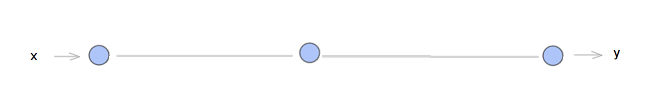
 the output will be
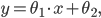
 and
and  . To construct a more advanced neural network which will be able to perform beter we add more nodes, connections and hidden layers, like in the image below.
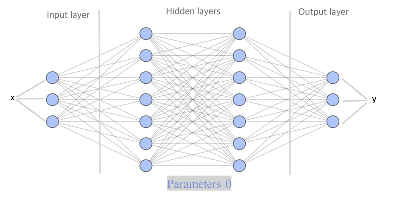
 is more advanced but can be still linear, in this case at each node in the hidden layers a linear equation is applied to the input from the previous nodes, and the output is forwarded to the next nodes following the connections of the network. The mathematical transformation you will apply to the input at each node can be chosen differently, you could also choose a quadratic function, or a sigmoid function.
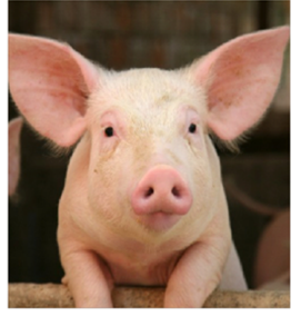
 on ImageNet (Deng et al., 2009) dataset. The left image is the original, and the right image is the original plus the noise image shown in the middle.
 (
( in the picture above) to the network, for some
  sufficiently small. Conventionally, it is anticipated for the classifier to place both
  in the same class if
  at node
  and an adversarial input
 . Although this mistake may seem small for each node, we have to see what happens when alls these small mistakes, in all the nodes in a layer, are combined with each other in the output. Suppose that the parameters
  , and that there are
  nodes in the layer. Then the total error will be increase by
  ! Which can get very large if
  with respect to
  . By calculating the gradient of the output of a neural network with respect to its input, an attacker can find the direction in which small changes to the input will cause the greatest change in the output. This is known as the gradient descent method.