Detection of bottlenecks is a topic that mathematicians have been working on for decades and which they continue to work on.
The fictitious Onebridge City, whose road network is depicted below, suffers from terrible traffic on a particular road, and it doesn't take a network scientist to see which one (the clue is in the name)! The circles represent important locations in the city and the lines joining the circles represent roads connecting the locations.
The bridge is of course the troublesome road because it acts as a “bottleneck”: if the bridge is closed for maintenance it is impossible to get between the two sides of the city and even when it is open it is likely to have a large volume of traffic and may become congested. Naturally, one would like to avoid such bottlenecks in this situation to improve the flow of traffic. In fact this problem arises whenever we wish to maintain a good flow of some sort, e.g. the flow of information in a computer network.
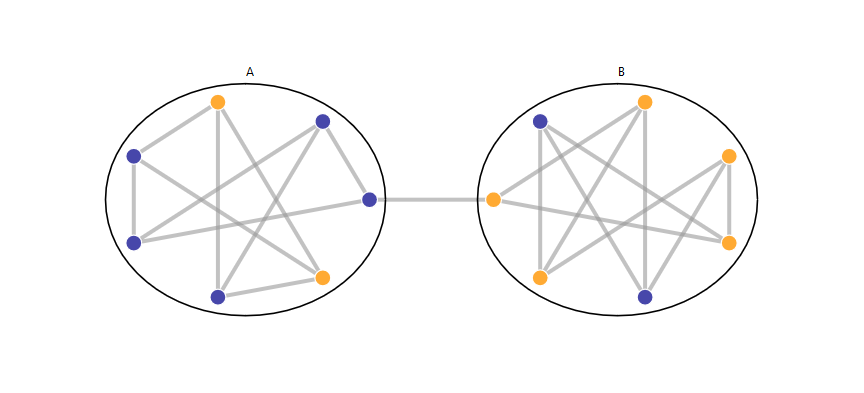
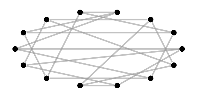
Consider the computer network below, where the circles represent computers and the lines joining them represent connections between the computers. Can you see any potential problems with this network?
In fact it is the same network as the road network of Onebridge city, just drawn differently! There is one connection whose failure would again result in the network becoming disconnected: can you see which one?
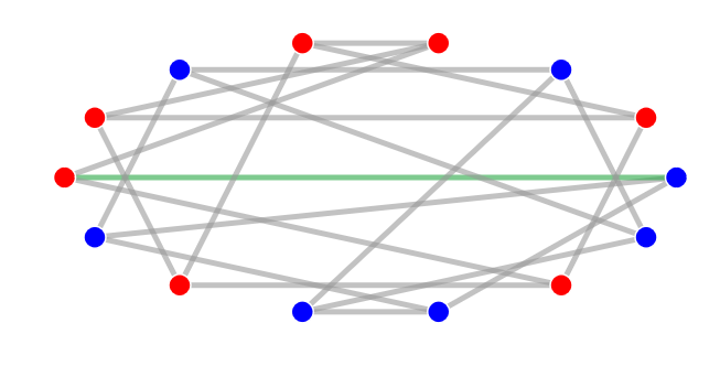
You can rearrange the circles in this network while preserving all the connections and obtain the network in the first picture. The green connection corresponds to the "bridge" in the first network.
Again, the bottleneck here is a vulnerability in the network because the failure of a small number of connections (just one in fact) results in two large parts of the network being unable to communicate with each other.
However, sometimes the presence of bottlenecks can be useful: in data networks such as social networks the presence of a bottleneck could indicate patterns in the data. I won't elaborate on this here, but in such situations we would also like to detect bottlenecks.
In order to avoid/fix bottlenecks, we must first be able to find them.
Finding the bottlenecks
It was easy to pick out the bottleneck in Onebridge City because the network was drawn in a suggestive way, but it was much harder in the computer network. It is harder still if the network is very large. This problem of detecting bottlenecks is one that mathematicians and computer scientists have been working on for decades and which they continue to work on. Using a beautiful analogy with nature, you will see and understand a powerful approach for finding these bottlenecks in networks: the approach is known as spectral partitioning. Sometimes, difficult problems in mathematics require a flash of ingenuity, but sometimes we need only look carefully at the world around us for inspiration!
Before explaining the approach for finding bottlenecks in networks, what exactly is a network and a bottleneck?
What is a network?
A network is a diagram (such as the ones above) consisting of a collection of nodes and links. The nodes are drawn as small circles and the links are lines between the nodes. So in the road network of Onebridge City, the nodes represent the locations in the city and the links are the roads between these locations, while in the computer network the nodes represent computers and the links are connections between the computers.
What is a bottleneck?
An important feature of the road network of Onebridge city is that it is connected, meaning that one can reach any location from any other using the roads. Thus we say that a network is connected if we can reach any node from any other node by traversing the links. For us, a bottleneck in a network is a small collection of links whose removal disconnects the network into two relatively large parts.
Here comes the main idea! It comes from the nature of heat flow, which is something we are familiar with from everyday experience. We all know that heat flows from hot objects to cold ones: for example think of a building with many rooms, some warm and some cold, with their doors left open. Over time, heat energy will flow along corridors from warm rooms to colder ones until eventually all of their temperatures are equal.
The main idea
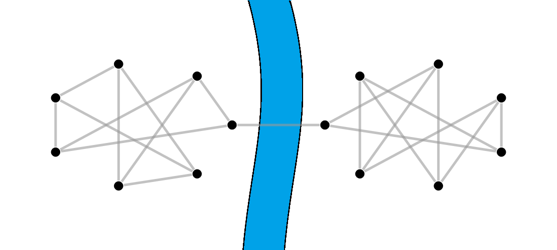
Suppose we would like to find the bottleneck in some given network. Imagine the network represents a building with the nodes being rooms and the links being corridors between rooms.
Imagine that we heat the rooms (i.e the nodes) to different temperatures and we let heat flow between them along the corridors (i.e. the links). Heat will tend to flow from hot rooms to cold ones until eventually the temperature of all rooms equalise (to the average of the original temperatures). However, suppose there is a bottleneck in our network as in the example below. Then we would expect that before the whole network equalises in temperature, we will see that the rooms on either side of the bottleneck, i.e. in region A (respectively region B) will first tend to equalise in temperature to the average in A (respectively the average in B) because A and B are “better connected” than the network as a whole. The animation below illustrates this. So examining the change in temperature over time will tell us on which side of the bottleneck each node is, so allowing us to identify the bottleneck.
It is this remarkably simple and familiar principle of heat flow that underlies many approaches to finding bottlenecks. We will now use the physical intuition from above to come up with an algorithm, i.e. a set of rules, to quickly locate bottlenecks in networks.
To keep things simple, we will focus on networks where each node has the same number of links (in the example we have seen every node has three links).
I will first describe how we can simulate heat flow in a network and then explain how to refine this into an algorithm for detecting bottlenecks.
Simulating heat flow in networks
Think again of our given network as a network of rooms in a building.
Randomly pick half the rooms (nodes) and heat them to a temperature of and give a temperature of to the remaining rooms. How do the temperatures of the rooms change over time? We use the following rule to update the temperatures.
For each room, to work out its new temperature, first look at its current temperature and look at the average temperature of its neighbours . The new temperature of the room will be the average of and . See the example below. The room (node) marked has a temperature of +1 and its neighbours have temperatures , , and . So . Since , the new temperature of the room is . We use this to update the temperature of all rooms simultaneously.
Once the temperatures of all rooms in the network have been updated we repeat step 1 with the new temperatures. We do this over and over again.
By clicking on the "Initialize weights" button in the example below, you will see that half of the rooms get a temperature of and the other half a temperature of . By clicking on "Update weights" you can see step 1 being applied to the example. Can you predict what will happen to the temperatures when you apply step 1 over and over again? You see that as we apply step 1 repeatedly, the temperatures of all the rooms tend to zero. Why is this? Step 1 represents the flow of heat through the network because the temperature of a room should become the average of its surroundings (i.e. its neighbours). Over many time steps the temperature of the whole network will equalise to the average value at the start, which was zero since we had an equal number of +1's and -1's.
While this nicely represents the flow of heat through the network, what we are actually interested in is not that the temperature equalises everywhere, but where equalisation is taking place first. So while all the rooms (i.e. nodes) are reaching a temperature of zero, we want to know which ones stay hotter for longer and which ones stay cold for longer. To do this, we introduce an extra step that allow us to “magnify” the process so we can see it better.
Magnifying the process
Here is the final refined algorithm that will allow us to find bottlenecks in our network.
As before, randomly pick exactly half the rooms of the network to have a temperature of and the remaining half a temperature of . Now we follow the same steps as before except that we introduce one new step (step 2) which “magnifies” the process for us. While step 1 tends to equalise temperatures, step 2 tends to separate the temperatures in a uniform way, and this will indicate which rooms (nodes) are staying hot or cold for longer.
For each room, to work out its new temperature, first look at its current temperature and look at the average temperature of its neighbours . The new temparture of the room will be the average of and . We use this to update the temperature of all rooms simultaneously.
Look at all the rooms with positive temperature and add their temperatures together to get a number . Reupdate each room's temperature from step 1 by multiplying it by where is the number of rooms in the network.
Repeat steps 1 and 2 with the reupdated temperatures over and over again.
What you will notice is that as we apply our rules over and over again, the temperature of the nodes will stabilise, that is, after a while they won't change very much. Try it with the interactive example below where we apply the steps above to the computer network from earlier. This time the temperatures of the nodes is indicated both by their colour and their horizontal position.
Now the stabilised temperatures of the nodes will reveal the bottlenecks of the network (if there are any). We already see this in the interactive example. The nodes on one side of the bottleneck end up with higher stabilised temperatures and those on the other side end up with lower stabilised temperatures. So to find the bottlenecks, simply check all the ways of splitting the nodes into those with high temperature and those with low temperature to see if you find a bottleneck. The stabilised temperature guides us as to how we should split the nodes to find the bottleneck; it hugely reduces the number of possibilitIes of splitting the nodes that we would otherwise have to check!
Conclusion
What you have seen is that identifying bottlenecks in networks is important, for example, to understand congestion/vulnerability in transport/communication networks (and there are many other applications not discussed here). Then you saw how the nature of heat flow inspires a powerful algorithm for quickly finding bottlenecks in networks. Mathematicians and computer scientists continue to refine and tweek these fundamental ideas to produce bespoke algorithms tailored for specific situations where detection of different types of bottleneck is required.
Finally I leave you with an interactive tool that applies the spectral partitioning algorithm above, but where you can choose the network! By clicking on two links in succession, you can replace them by two new links and you can repeat this to create new networks to apply the algorithm to. The link in green is one of the two links you want to replace while the links in red are not allowed to be chosen. You can chose one of the remaining gray links as the second link to be replaced.
Both animations in this article were made by Martijn Gösgens.
Rafael Prieto-Curiel is a mathematician and a faculty member at the Complexity Science Hub in Vienna, Austria. His research focuses on crime, mobility, migration and urban dynamics. We interviewed Rafael to learn about his story.
We participated in a three-day science fair in Brussels, called Science is Wonderful!, for which we designed an interactive booth aimed at introducing young people to network science. Here's what we learned!
Using data analytic techniques and Artificial Intelligence you can analyse data from hospitals and discover hidden patterns that allow us to often predict (within a margin of accuracy) failures before they happen. When a failure is predicted, we issue an alert and we plan for preventive maintenance by an expert engineer.
One of the main building blocks of modern AI-tools are artificial neural networks, abstract models inspired by the structure and functions of biological neural networks which enable machines to "learn". In this article, I will discuss some thoughts on this topic.
 and give a temperature of
  to the remaining rooms. How do the temperatures of the rooms change over time? We use the following rule to update the temperatures.
 and look at the average temperature of its neighbours
  . The new temperature of the room will be the average of
  has a temperature of +1 and its neighbours have temperatures
  . Since
  , the new temperature of the room is
  . We use this to update the temperature of all rooms simultaneously.
 . Reupdate each room's temperature from step 1 by multiplying it by
  where
where  is the number of rooms in the network.