Random walks are popularly described as a drunkard’s path down the streets. What happens when the streets also start to move?
I still vividly recall when I heard about a random walk for the first time. The lecturer told us to imagine a company of drunken students who wander in the streets, and whenever they come to an intersection one of them just spins around and they all go down the path that ends up being in front of the spinning student's eyes. Let us try to follow in the footsteps of our intoxicated friends.
When we describe this random walk, are details like the names of the streets important? It seems not, all that matters are the intersections and the streets that connect them. In an abstract setting, we will call these streets edges; intersections will be called vertices and these two together will form a graph. Also, do we need to watch our company all the time? Not really, all the interesting things happen at the intersections, so let’s just watch our walkers there. This introduces a natural time step in the process that we follow.
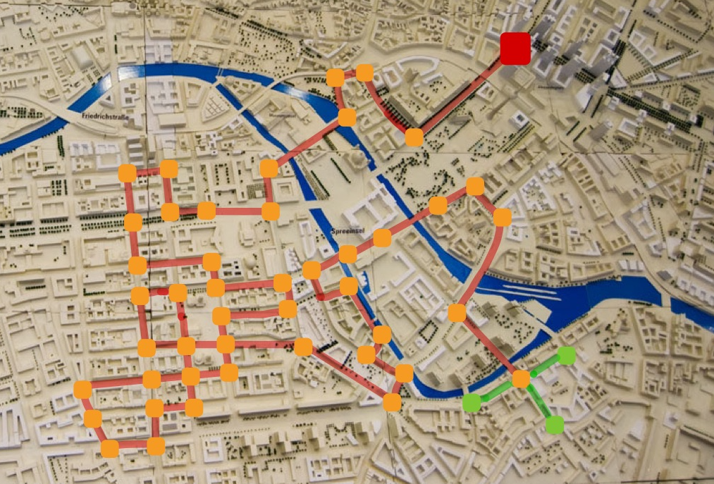
Figure 1: An example of a (non-backtracking) random walk. The red square marks the starting position, red lines denote the edges the random walk has traversed and orange square mark the intersections. In green are the possible edges the walker can take and the intersections he might end up at. Created on top of Sebastian Niedlich’s photo “City Planning V”, licensed under CC BY-NC-SA 2.0 license.
An abstract random walk – one of the most classical mathematical models – is just the story described above with all the superfluous details removed. Random walks have found use in the analysis of gambling, the stock market (one could argue that these two are the same), biology (for example Brownian motion), and many other scientific fields. This is the beauty of mathematical abstraction – it is not self-serving, rather it allows us to reason about an abstract model that can be later applied to stock prices, moving pollen particles, or drunken adventures.
Now, let us return to our story. Imagine we want to bring the drunken party back home. But to do that we must first find them! Where do we start looking? Well, if they have just left, then a suitable place to look would be at the intersection in front of the pub. In a while after that, our walkers will be at one of the intersections down the street from the pub, with no preference for any of them. For example, if there are 3 intersections around the one where the pub is, then they could be at any one of them with a probability 1/3. But if we wait for too long then our characters can be just about anywhere in the city, and the fact that we know where the starting point was, will no longer help us – we have lost them.
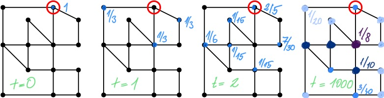
Figure 2: Distribution of the random walk at the start of the walk and then after one, two and way too many steps. The red circle marks the starting position. Blue dots represent the intersections where the random walker may end up being and the numbers next to them represent the probabilities of a random walker being there. In the final figure the probabilities are proportional to the number of streets connected to any given intersection. Different probabilities in this final figure are colour-coded with the respective value written in corresponding colour.
Could this be again some mathematical abstraction dressed as an alcohol-fuelled story? The pub here marks the initial position. The list of probabilities of our students being at any given intersection after a given amount of time is called a distribution of the random walk, see Figure 2. If we wait long enough this distribution will be no longer influenced by the initial position – the stationary distribution has been reached. And finally, the time after which we have waited for too long and the distribution starts to closely resemble its stationary version is called the mixing time. We can tie all these new objects together by saying that after the mixing time has elapsed, the random walk has reached its stationary distribution and is no longer affected by the initial position.
Mixing times are important for physics, cryptography, or even card shuffling. Concerning card shuffling, you can ask how many shuffles you need to get a truly random deck. But this is still an old and well-established topic. To get into new territory, I will need to deliver on my promise from the title and make the life of our inebriated friends much more complicated – their world will start moving! The rest of this article is driven by the following question:
What happens to our random walker when the streets start changing which intersections they connect to as time goes by? Do we have more time before we lose them or the other way around?
Let me paint you a picture of this: from time to time some of the streets get broken in halves and these halves reconnect in such a way that these streets suddenly lead to a different intersection than before. This is a true game-changer; just imagine how would you react if you suddenly saw a street change where it leads to! In its full generality, this is an unsolved problem.
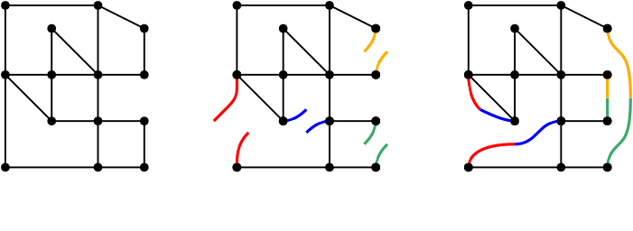
Figure 3: On the left, we have a graph in its initial configuration. On the middle figure some of the streets are broken in halves, ready to be repaired to a different segment. In the final picture we see new connections arising after rewiring has taken place.
To make the situation a little bit more tractable let me simplify the setting with two assumptions:
Assume that the streets that get rewired are chosen at random from all the streets in the city – there is no bias, omission or “malicious actors” involved. More technically, we would say that the edges that get rewired are chosen uniformly at random from the entire edge set.
Furthermore, assume that the students random walk is without immediate backtracking. This means that they will never go back the same street crossed in the previous step.
The first assumption will guarantee that the rewiring mechanism can get us truly anywhere. Once a street gets broken up it can be rewired with any other street – there are no preferred or disliked possible pairs. The other assumption makes our group of students go boldly forward, so they will never second-guess the previous move and move back to their previous position. In this setting, how much time do these delirious students need to get lost?
The key here is to realise that as long as the drunkards do not come across a street that got influenced by this process of breaking up and repairing, they are basically still walking on the initial graph. So, from an outside point of view this dynamic situation is the same as if they just walked on the initial graph (consisting of the streets as they were before he got into the pub) and occasionally got thrown off into an absolutely random part of the city.
Using the realisation above we can observe this voyage from two points of view. On one hand, the students believe that the streets are dancing around, because after traversing only one street they emerge somewhere where they could not have ended up according to their sober memories of the city plan. On the other hand, an observer whose experience is closer to our everyday reality sees that the students simply made use of a different mode of transportation, for example a night bus. Both of these experiences are perfectly valid descriptions of what is going on and they are actually the same all the way until the students step over what seems to be a rewired street.
Intuitively we see that the first time the students cross a street that they “definitely, literally” saw moving is a good candidate for a mixing time. Why is that? Thanks to our first simplifying assumption we know that the rewiring can get you anywhere. So, from the point of view of a sober observer watching the streets in their usual configuration, the walker has just been thrown to a random part of the graph. You could hardly imagine getting thrown more off-course than that! Even on a formal level, this intuition about the mixing time turns out to be true.
Here we could easily get side-tracked into the direction of many fascinating details, but let’s get back to our original question: will our friends get lost faster than in the static situation? As usual, the honest answer is: “It depends”. We see that the random walk will become mixed the moment it steps over a rewired edge. If this happens sooner than the mixing would happen in the static situation then there is clearly a speedup. But what if our company does not meet any rewired street? Well, in that case the mixing time will be exactly the same as it would be on a static graph – because the entire walk happened on edges that have remained the same as in the static initial graph.
So, we see that the mixing is at least as fast as in the static situation. Is it possible to dream up a mechanism that would still allow the walkers to get lost but possibly slower than in the static case? This is not clear. While there are some examples when a slow-down of mixing due to graph dynamics can occur, these are much more artificial than the one we explored here. Is there a reasonably natural dynamic that exhibits this phenomenon? I cannot answer that question.
The final point I want to make here returns us to the beginning of this article. All the images and intuition here can be abstracted into the language of graphs, edges and random processes. This way we see that the same results that hold for a group of students stumbling around in a changing world also hold for, e.g., the internet. The internet is a stereotypical real-life example of something that can be reduced to a dynamically evolving graph. In a more web-flavoured version of this story we would be following a crawler programme from your favourite web-search company and instead of streets and intersections we would be talking about hyperlinks and pages connected by them.
More generally, there are lots of real-life processes that resemble a random walk and happen on a dynamic structure well-modelled by a dynamic graph. So maybe next time you end up with a problem that feels like a random movement of a hallucinating person, enlist a mathematician for some professional advice.
Together with Arnaud Bom from Analytic Storytelling, we decided to promote some of the articles on the Network Pages because of the creative writing techniques the authors used. We want to share these writing tips with you so that you can apply them in your writings!
In the city of Utrecht there are four wall paintings of Dutch physisists. Do you know which ones? In this short blog post we want to take you on a virtual bike ride in the city of Utrecht.
On a quiet afternoon, professor Meth is working in her office in Leiden on some tantalizing mathematics problems. Suddenly, someone knocking on her door nervously disrupts the silence.
In this article, dear reader, I am going to show you in which way the development of your opinion during the last political issue, the spread of a virus among your acquaintances during the current pandemic, and the alignment of some particles lying inside the device from which you are reading this article are extremely comparable phenomena.