Wireless communication networks play a crucial role in connecting laptops, smartphones, sensors and countless physical devices, and in exchanging data among persons, computer brains and other parts of our information society. Due to the immense size and intricate infrastructure it is impossible to have a central coordination of the data traffic in these networks. Therefore, so-called random-access algorithms are typically used, allowing individual users to direct the data streams in an autonomous way. This article describes stochastic particle models to understand the macroscopic behaviour of these networks and improve their performance.
Wireless networks and particle models
Data is increasingly being transmitted wirelessly, because of improvements in ease of use, range and flexibility when compared to wired networks. A defining characteristic of wireless communication is that the signals are transmitted in all directions, instead of only towards the intended receiver. Therefore, the numerous signals in large-scale networks can distort each other as the result of interference. To prevent or decrease such interference it is therefore important to make sure that nearby users of the network do not transmit data at the same time. To this end, wireless networks rely on algorithms that control the activity of the users.
If we consider a group of wireless users, for example devices such as laptops, tablets and smartphones, the positions and activities of these devices form the network. Each device has its own data buffer and generates data, which the user wants to transmit to a certain receiver using wireless communication. The network is stable when all individual buffers are stable, and the global perspective of the network as a whole is therefore closely intertwined with the local perspective of individual users.
We assume that the activities of the users are controlled by local algorithms, allowing each user to determine when these data are transmitted, relying only on local information. An example of such a local algorithm is implemented in the so-called IEEE 802.11 protocol, which is at the heart of WiFi networks such as the ones we use every day at work, on the train and at home. The algorithm roughly works as follows. The capacity is divided among nearby devices using a lottery. This game of chance is played, say, every millisecond, and the device with the winning lottery number is allowed to transmit data during that millisecond.
An interesting refinement of this protocol, as we will discuss later, is the use of a weighted lottery. The more data awaiting transmission in the buffer of a device, the more lottery tickets this device gets to take part in the lottery. In this way, the system stabilizes more effectively. Buffers that are less full win less often and therefore fill up, while the fullest buffers get the opportunity to be emptied.
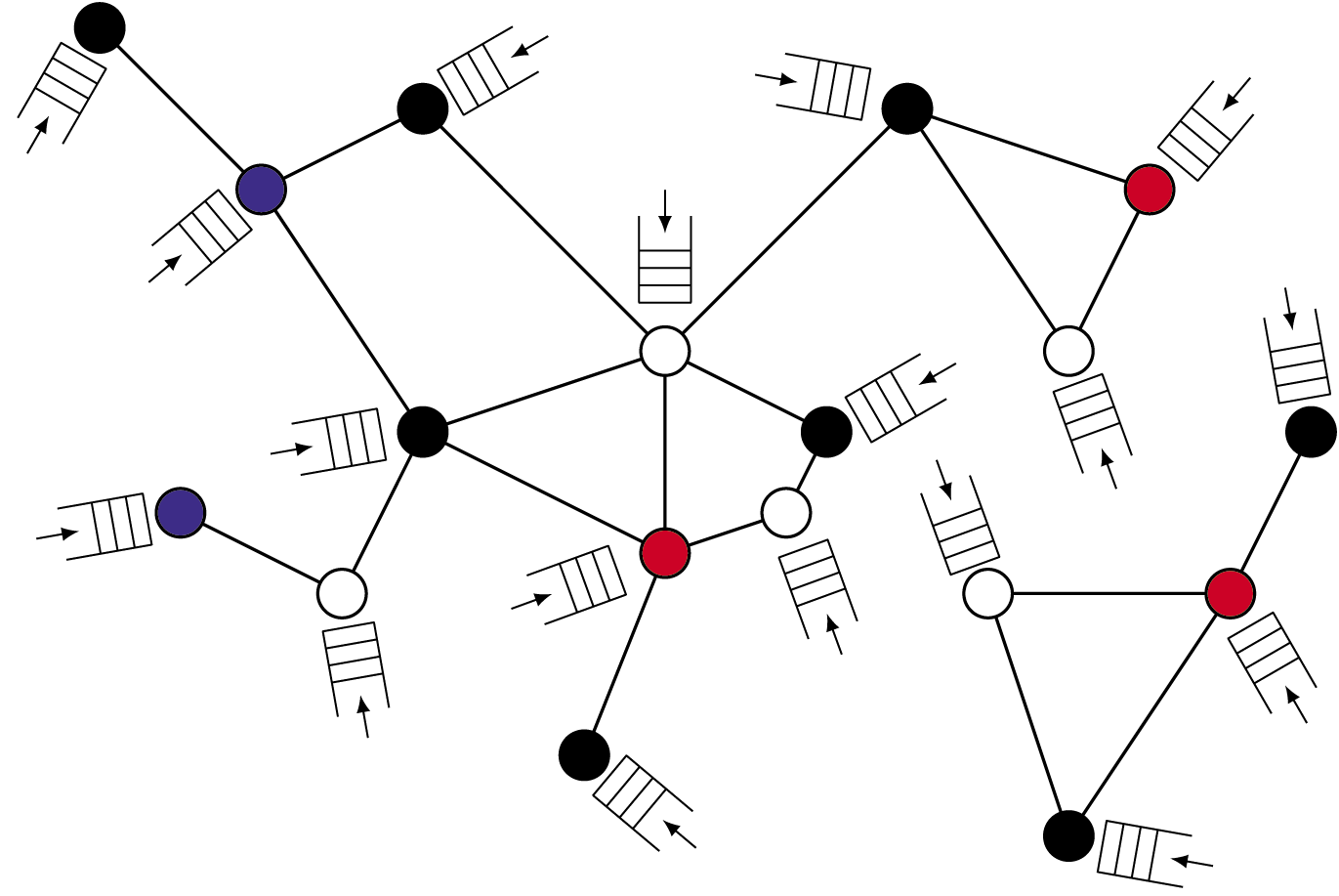
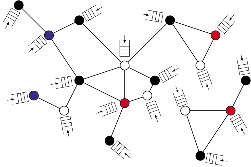
Figure 1: An interference graph of wireless users and their buffers.
If we consider the wireless networks and local algorithms from a more abstract point of view, we arrive at a probabilistic particle model on a graph. The graph consists of N nodes (the users in the network) and two nodes that are connected by an edge cannot be active (i.e., send data) simultaneously. Think, for example, of users who are in close vicinity of each other and could therefore distort each other's signals. This graph is called the interference graph. A local algorithm, slightly stylized, could operate as follows within this graph:
Every node gets a timer, set to go off after an exponential time, with mean .
As soon as its timer goes off, the node attempts to activate and transmit data. The node will, however, first need to check if none of its neighbours in the graph is already active.
If none of its neighbours is active, the node will transmit data for an exponential time, with mean 1.
If at least one neighbour is active, the node whose timer went off will not activate, instead trying again after another exponential time, with mean .
In this way we arrive at a stochastic network consisting of nodes that are alternately active and inactive. The local and also random algorithm described above ensures that all nodes have a regular opportunity to transmit something, and prevents neighbouring nodes from being active at the same time. The parameter is a measure of the aggressiveness of the algorithm: when is small, the nodes will wait for a long time in between subsequent activation attempts, and relatively few nodes will be active at the same time. In the context of random-access networks, we call this parameter the activation rate.
Because of the randomness of the algorithm described above, such networks are called random-access networks in the research literature. Because of the assumptions of exponentiality, random-access networks can be described in terms of stochastic models known as interacting particle models. These particle models are used often in fields such as mathematics, physics and chemistry (see also [7]). For example, in statistical mechanics, magnetism is described in terms of the Ising model, a particle model where the particles are magnetic dipoles whose spins are either directed upwards (spin state ) or downwards (spin state ). The particles in random-access networks have a state (inactive) or (active). In both particle models the particles have some form of interaction. While magnetism gives rise to ferromagnetic interaction (neighbouring particles prefer the same direction), the interaction in random-access networks is anti-ferromagnetic: the neighbours of a particle in state will always be in state 0. This strict type of interaction is sometimes called hard-core interaction and, besides in random-access networks, can also be applied to molecular gases where the molecules do not allow each other to come close [10].
Let denote the state of node at time of the particle model that includes governed by this hard-core interaction. We introduce and remark that is a Markov process. The long-term behaviour of this process has been studied extensively in literature, especially its limiting distribution the distribution of limits . This distribution describes for each possible network state the frequency with which this state occurs in the long term. A state is a combination of active and inactive nodes, such that . The limiting distribution of limits can be expressed elegantly in terms of the network parameters: \begin{equation} \label{eqn:limiting} \pi(\boldsymbol\omega) = Z^{-1} \prod_{i=1}^N \nu^{\omega_i}= Z^{-1} \nu^{|\boldsymbol\omega|}, \end{equation} where is the normalisation constant that ensures that the probabilities add up to .
The set of states that the network can take consists of all independent sets of the interference graph. An independent set is a subset of nodes of the graph, no two of which are connected by an edge. (For convenience we assume that the wireless network only has one frequency channel available. If the network has multiple frequency channels, the role of the independent sets is taken over by the colouring of the interference graph, see for example [11].)
Finding the independent sets of a graph, especially its largest independent set, is one of the classic problems in graph theory, and is known to be NP-complete. So, despite the elegant and apparently simple structure, the limiting distribution in (1) can be very difficult to calculate, in large networks with large interference graphs, as all independent sets need to be found to determine . This is an illustration of the striking fact that while the random-access network can be controlled locally, its behaviour and performance are described in terms of global properties such as the independent sets. In this article we discuss two crucial performance measures for random-access networks: long-term throughput and short-term delays. The mathematical analysis of the particle model provides insights into these performance measures and is based on techniques from probability theory applied to the class of Markov processes, to which the particle models belong.
Throughput of wireless networks
The long-term throughput is defined as the amount of data that can be transmitted on average per unit of time, expressed for example in bits or packets per second. Of course, users are best served having a high throughput. For the moment, we assume that nodes always have data packets to transmit and so will activate whenever the clock times and neighbour activities allow them to. Later on we will relax this assumption.
We assume that nodes transmit one packet when activated. The throughputs of the various nodes in the network exhibit strong interdependencies because of the fact that neighbouring nodes in the graph are prevented from being active simultaneously. Consequently, when a node has a large throughput and transmits many packets, its direct neighbours will have less opportunity to become active and, as a result, will experience a lower throughput.
This competition among nodes is central in the analysis and design of wireless networks. This is because the nodes have to share the capacity of the wireless network, and it is important that this happens in a fair or acceptable way. For example, an obvious question is: ''How do we design a wireless network in which all nodes have the same throughput?''
To answer this and similar questions, we can utilize the limiting distribution . The throughput of node can be expressed in terms of the limiting probabilities as follows: \begin{equation}\label{eqn:throughput} \theta_i := \sum_{\boldsymbol\omega:\omega_i=1} \pi(\boldsymbol\omega)=Z^{-1} \sum_{\boldsymbol\omega:\omega_i=1} \nu^{|\boldsymbol\omega|}, \end{equation} with the vector of the throughputs of all nodes. The summation is thus over all states in which node is active.
In [9], detailed simulations are used to show that the throughput of the particle model approximates the throughput of wireless networks in practice remarkably well – despite the fact that for instance signal strength, collisions and fluctuations of the wireless signal are not taken into account in the particle model that is applied to the graph. Since the particle model describes reality so well, it can be used to reduce the differences of the per-node throughputs.
First, notice that different throughput values differences occur for almost all interference graphs. Consider for example a network of nodes on a line, where each node blocks its immediate neighbours when it becomes active. Figure 2 shows the throughput of each node as calculated using for different values of ν. The outermost nodes of the network have the highest throughput, as they have only one neighbouring node, and can activate more often than the other nodes. Each line corresponds to a certain value of ν, with the oscillation increasing with increasing ν. Using it is easy to see that when for all odd-numbered nodes, and for all even-numbered nodes.
Figuur 2: Throughput of a linear network of 9 nodes for different values .
One way to fix these unequal or unfair throughputs is by assigning different activation rates to nodes. If node has an activation rate , and , then can be rewritten as \begin{equation}\label{eqn:throughput2} \boldsymbol\theta(\boldsymbol\nu) := \Big(Z(\boldsymbol\nu)^{-1} \sum_{\boldsymbol\omega:\omega_i=1} \prod_{j=1}^N \nu_j^{\omega_j}\Big)_{i=1,\dots,N}. \end{equation} Consider, for example, the linear network of nodes, where active nodes block their immediate neighbours. Define as a constant and as the number of neighbours of node . It can be easily shown (see [15]) that, when we assign activation rate \begin{equation} \nu_i = \alpha(1+\alpha)^{\gamma(i)-\gamma(1)}, \quad i=1,\dots,N, \end{equation} to node , every node will have a throughput of \begin{equation} \theta_i = \frac{\alpha}{1+2\alpha}, \quad i=1,\dots,N. \end{equation}
As , and voor , we see that the outermost nodes are assigned a lower activation rate than the other nodes. This is intuitively clear, as it compensates for the high throughput of the outer nodes in the case all activation rates are the same.
Finding activation rates such that all nodes in a linear network will have the same throughput is just one example of a much larger class of problems: given a general interference graph, how should we choose the activation rates to achieve a certain vector of throughputs? To answer this question, we introduce the set , containing all possible combinations of throughputs that can be achieved by selecting the right activation rates. This set of course depends on the structure of the interference graph, and can be interpreted as the range of the function introduced in . This range can be characterised as the interior of the convex hull of all possible independent sets of the interference graph.
Next, suppose that γ∈Γ is a vector of the throughputs values we wish to achieve. We are now looking for the solution ν=ν(γ) of the system of equations
Next, suppose that is a vector of the throughputs values we wish to achieve. We are now looking for the solution of the system of equations \begin{equation}\label{eqn:inverse_problem} \boldsymbol\theta(\boldsymbol\nu) = \boldsymbol\gamma. \end{equation} This is not a simple problem in general, due to the complex behavior of the function .
The first step towards solving is to determine that is globally invertible, so for every vector , exactly one solution to exists, see [14]. In contrast to the example of achieving equal throughputs in a linear network, it will be in general impossible to find a closed-form expression for . Instead, we can apply for example numerical methods to solve the system.
There is, however, an alternative approach to determine , in which the nodes adapt their own activation rate based on the difference between the realised throughput and the desired throughput. To this end, time is divided into intervals of duration , At the end of each interval, the activation intensities rates can be adapted. Let , and adapt modify this recursively as follows: \begin{equation}\label{eqn:JW} r_i(j+1) = \big(r_i(j) + \beta(j)\big(\gamma_i - \hat{\theta}_i(j)\big)\big)^+, \end{equation} where is the empirical throughput in the -th interval. It can be shown that for the right choice of , the recursive series indeed converges to a solution such that , [8]. This is a remarkable result, as the adjustment modification can be calculated separately by each user, and the nodes arrive in a fully distributed way at the correct throughputs values despite the complex interactions in the network. Like the simple algorithm described in the previous paragraph, is a local algorithm.
Congestion and delays
The basic model as discussed in the previous sections is based on the assumption that there are always packets available for transmission in the buffers of the various nodes. In reality, the buffers will not be 'saturated' like this, but contain varying numbers of data packets as a result of natural fluctuation in the generation and transmission of data packets with time. In particular, the buffers will be completely emptied from time to time. It is important to analyse the stochastic behaviour of the buffer contents, as well as the time a packet spends inside the buffer in between generation and transmission. This sojourn time, or delay, offers a crucial measure for the performance of wireless networks as experienced by users.
For the remainder of this section, we assume that data packets are generated at node i according to a Poisson process with rate . To model the stochastic behaviour of the buffer contents, we introduce , where denotes the number of packets awaiting transmission or being transmitted at node at time . Despite the fact that, now, buffers now sometimes do not contain any packets, we first maintain the assumption that the nodes are constantly competing for the medium and always activate when they get the opportunity to do so. This assumption implies that the activation process of the various nodes is not influenced by the state of the buffers, and therefore maintains the equilibrium distribution . It can then be shown that the Markov process is positive recurrent when for all nodes . The process is also Markovian, and behaves as a so-called quasi-birth–death process, for which the equilibrium distribution can be determined numerically by using so-called matrix geometric methods.
To gain some qualitative insight, we now consider a regime in which the arrival rates are relatively high. In order to guarantee stability for such arrival rates, the throughputs also need to be relatively high, which in turn requires high activation rates . Such a regime is not only interesting theoretically but also relevant from a practical point of view. This is because a relatively high load can result in long delays and lower quality of the wireless service, while delays do not pose an essential problem in case of lower arrival rates.
To clarify the global situation, we look at a symmetric scenario in which all nodes have the same arrival intensities rates and activation intensities rates . We also focus specifically on an interference graph consisting of a square lattice of dimension , as illustrated in Figure 3.
Figure 3: Even and odd configurations of a network with a lattice structure.
In the case of ‘periodic’ boundaries, where the lattice becomes a torus, the nodes at the periphery experience not only interference by direct neighbours but also from the corresponding nodes on the opposite sides of the lattice. Both for ‘open’ and periodic boundaries, it is easy to see that there are two maximum configurations of size , corresponding to the white and black fields of a chess-board, see Figure 3. For convenience refer to the maximum configurations and the corresponding nodes as 'even' or 'odd', respectively.
In case of high activation rates, the system will almost always be in one of the two maximum configurations. Transitions between both maximum configurations rarely occur, i.e. on a timescale of the order of O for large values of , where the exponent equals or , respectively, in the case of an open or periodic boundary. As a result, nodes that are not in the current active configuration will have no opportunity to transmit packets for a long time. For example, when the even configuration is active, packets arriving at the odd nodes will accumulate until at a certain time a transition occurs to the odd configuration, and the odd nodes will be given the opportunity to transmit a substantial number of packets in a row. The sequence of long periods of accumulation and transmission implies that the number of packets at an individual node evolves according to a saw tooth-like pattern, as illustrated in Figure 4. The amplitude of the saw tooth pattern is proportional to the associated timescale, and therefore roughly of the order O for large values of .
Figure 4: Buffer contents as a function of time for a lattice network.
It is easy to verify that for both the open and periodic boundaries, and are necessary conditions to ensure the stability of the system. We therefore conclude that the average number of packets contained in the buffer of an individual node is at least of the order of O when the arrival rate approaches the critical value [16]. Because of Little's Law, the average delay of a packet has the same order of magnitude. It is important to compare this scaling with the usual situation in conventional queueing systems where the average delay should be of the order of O. See for example [5] for an introduction to queueing theory. In other words, the slow transitions between the rigid maximum configurations have a strongly negative effect on the scaling of the number of packets and the delay, which furthermore gets worse with the size of the network as reflected by the exponent .
More advanced algorithms
The model outlined above relies on the simplification that nodes always activate when they get the chance, even when the buffer does not contain any packets. From a practical point of view it is obviously more likely that nodes will temporarily refrain from competing for the medium until the next packet that needs to be transmitted.
As a consequence, the state of the buffers as represented by the process is not only determined by the activation process but conversely also influences , which therefore loses the equilibrium distribution . Although the process remains Markovian, the interaction between both components gives rise to serious complications in the mathematical analysis.
Even necessary or sufficient conditions for positive-recurrent behaviour are in general not easy to characterise. As it seems reasonable that nodes with empty buffers withdraw from the competition for the medium, it would be obvious to assume that the earlier condition for all nodes would be sufficient to guarantee stability. Surprisingly though, this turns out not to be the case. To illustrate and explain this, we consider a network of nodes and interference between nodes and , and , and , and and . If for instance node has a very low arrival rate, it will very rarely engage in competing for the medium. Node is therefore nearly isolated in competing with nodes 1 and 3, and in a disadvantaged position. This means that even if node 2 has packets available for transmission all the time, (and nodes 1 and 3 have rather high arrival rates), the throughput received for node can be substantially lower than the value for the case when the buffers of all four nodes would be in a saturated condition. As a result, instability can occur at node when the arrival rate is only slightly lower than the value [13].
The subtle relations among neighbours in the previous simple example are typical for the complex interactions among the various nodes. As a consequence, characterising the necessary and sufficient conditions for positive-recurrent behaviour is in a way as difficult as fully determining the equilibrium distribution of the process . For Markov processes without a specific (product-form) structure and with a state space that is infinite in multiple dimensions, there are few general results available. It turns out that for complete interference graphs explicit conditions for so-called rate stability can be determined [13]. For all other interference graphs it is difficult to deduce closed-form conditions for overall stability. The results for complete interference graphs do imply partial stability conditions for certain subsets of nodes [6].
The description above assumes that the activation rate of node is zero when the buffer is empty and equal to a constant when the buffer is non-empty. So-called queue-based algorithms offer an interesting generalisation in which the activation rate of node at time is a general (typically increasing) function of the number of packagespackets contained at that time by the buffer. A related variation of the basic algorithm concerns node transmitting not just one packet but, when the transmission ends at time , immediately sending a next package packet with probability , where is a typically decreasing function and . For these model variations the Markovian character of the process is maintained as well.
In the special case that , it is possible to determine the equilibrium distribution of the number of packets for several special choices of the functions and [2]. The ratio of the functions and determines to a large degree the qualitative behaviour in the regime where the arrival rate approaches the critical value . Although the number of packets in such a regime inevitably grows, there are three distinct asymptotic regimes depending on whether the ratio increases super-linearly, linearly or sub-linearly with q. Because of Little's Law, the same three-way split occurs in the growth behaviour of the magnitude of the delay of the packets.
It needs no explanation that in case of nodes, the equilibrium condition of is even less analytically tractable than in the scenario described earlier, where and .. In the light of this observation it is even more remarkable that very explicit stability conditions have actually been identified, even though the proofs are very advanced. For a broad class of and functions it was shown that the necessary condition that the vector of arrival rates is part of the convex hull is also sufficient for stability [11]. This ground breaking result demonstrates that distributed algorithms, if constructed carefully, have the potential to match the throughput and maximum stability of complex centralised mechanisms.
This important fact raises the question whether these algorithms are also capable of conquering the adverse delay scalings described earlier. Unfortunately, the scaling does not appear to improve significantly, specifically for the class of functions which were shown to achieve the optimal throughput and maximum stability [3]. To a certain extent, this drawback is unavoidable, as reducing delays implicitly requires that the maximum configuration can be quickly found. Because the latter problem is NP-difficult, it should be considered highly unlikely that the unfavourable scaling of delays can be improved significantly using queue-based algorithms.
Extensions and remarks
Particle models have been used since the 1980s to analyse random-access networks [4] and have provided valuable insights into the behaviour of these networks. The adaptive algorithms described here offer interesting possibilities to make the current generation of random-access networks more flexible and robust. Although the models described succeed in capturing the most relevant characteristics of wireless networks, several phenomena from practice are not modelled explicitly. We conclude this article by discussing two of these phenomena, which, should they be turned into a mathematically tractable form, would advance both wireless networks in practice, and the development of mathematical theory.
Mobility and user dynamics.
The interference graph forms the basis of the mathematical study of random-access networks, and is always assumed to be static. In practice, however, we see that the network is in motion. That is to say, the users of the devices move, making the structure of the network dynamic. In addition, users will also join the network and, after some time, leave it. A static interference graph is therefore nothing more than a snapshot of the state of the network. This poses an additional challenge to the adaptive algorithms. Indeed, instead of converging slowly to a desired vector of throughputs, this vector will change over time. The question then is not whether we can find algorithms that converge to certain throughputs, but how well we can follow the ever changing throughput targets, and hence how fast we can respond to changing circumstances.
Forwarding of packets.
The queueing models described before concern so-called single-hop scenarios, where each node has its own packet arrival process, and a packet exits from the network as soon as it is transmitted. In reality, sent packets are often forwarded to other nodes, for example in order to transit the network. This reinforces the interdependence between nodes, as the arrival processes of new packets at a node now also depend on the activation process of its neighbours. It seems far from feasible to exactly analyse such multi-hop scenarios, and it will be necessary to focus on approximations and scaling limits to arrive at mathematically tractable results.
References
This article was published in the "Nieuw Archief voor Wiskunde" 5th series, part 3, number 16. The Network Pages acknowledges NAW for its permission.
N. Bouman, S.C. Borst, O.J. Boxma, J.S.H. van Leeuwaarden, Queues with random back-offs, Queueing Systems 77(1) (2014), 33-74.
N. Bouman, S.C. Borst, J.S.H. van Leeuwaarden, Delay performance in random-access networks, Queueing Systems 77(2) (2014), 211-242.
R.R. Boorstyn, A. Kershenbaum, B. Maglaris, V. Sahin, Throughput analysis in multihop CSMA packet radio networks, IEEE Trans. Commun. 35(3) (1987), 267-274.
O.J. Boxma, S. Kapodistria, M. Mandjes, Performance analysis of stochastic networks, Nieuw Archief voor Wiskunde 5/16(3) (2015), 193-200.
F. Cecchi, S.C. Borst, J.S.H. van Leeuwaarden, Throughput of CSMA networks with buffer dynamics, Perf. Eval. 79 (2014), 216-234.
D. Garlaschelli, F. den Hollander, A. Roccaverde, Complexe netwerken vanuit fysisch perspectief, Nieuw Archief voor Wiskunde 5/16(3) (2015), 207-209.
L. Jiang, J. Walrand, A distributed CSMA algorithm for throughput and utility maximization in wireless networks, IEEE/ACM Trans. Netw. 18(3) (2010), 960-972.
.C. Liew, C.H. Kai, H.C.J. Leung, P.B. Wong, Back-of-the-envelope computation of throughput distributions in CSMA wireless networks, IEEE Trans. Mobile Comput. 9(9) (2010), 1319-1331.
J. Sanders, Atomaire gassen en draadloze netwerken, STAtOR 15(1) (2014), 9-12.
D. Shah, J. Shin, P. Tetali, Medium access using queues, In: Proc. FOCS 2011.
D. Shah, D. Tse, J. Tsitsiklis, Hardness of low delay network scheduling, IEEE Trans. Inf. Theory 57(12) (2011), 7810-7818.
P.M. van de Ven, S.C. Borst, J.S.H. van Leeuwaarden, A. Proutière, Insensitivity and stability of random-access networks, Perf. Eval. 67(11) (2010), 1230-1242.
P.M. van de Ven, A.J.E.M. Janssen, J.S.H. van Leeuwaarden, S.C. Borst, Achieving target throughputs in random-access networks, Perf. Eval. 68(11) (2011), 1103-1117.
P.M. van de Ven, J.S.H. van Leeuwaarden, D. Denteneer, A.J.E.M. Janssen, Spatial fairness in linear random-access networks, Perf. Eval. 69(3) (2012), 121-134.
A. Zocca, S.C. Borst, J.S.H. van Leeuwaarden, F.R. Nardi, Delay performance in random-access grid networks, Perf. Eval. 70(10) (2013), 900-915.
During our teenage years, everything changes. It’s no surprise that our brain does too. But how do we make sense of this transformation? Is there a way to quantify it? Networks might just be the answer.
One of the main building blocks of modern AI-tools are artificial neural networks, abstract models inspired by the structure and functions of biological neural networks which enable machines to "learn". In this article, I will discuss some thoughts on this topic.
Think of a local car dealer selling cars in your region. To make sure new cars are delivered on time a whole mechanism involving various people, factories, and transport companies, must operate in coordination. This is a highly complex process where mathematics plays an important role.
Rafael Prieto-Curiel is a mathematician and a faculty member at the Complexity Science Hub in Vienna, Austria. His research focuses on crime, mobility, migration and urban dynamics. We interviewed Rafael to learn about his story.

 .
. is a measure of the aggressiveness of the algorithm: when
  is small, the nodes will wait for a long time in between subsequent activation attempts, and relatively few nodes will be active at the same time. In the context of random-access networks, we call this parameter the activation rate.
 ) or downwards (spin state
  ). The particles in random-access networks have a state
  (inactive) or
  (active). In both particle models the particles have some form of interaction. While magnetism gives rise to ferromagnetic interaction (neighbouring particles prefer the same direction), the interaction in random-access networks is anti-ferromagnetic: the neighbours of a particle in state
  denote the state of node
  at time
  of the particle model that includes governed by this hard-core interaction. We introduce
  and remark that
  is a Markov process. The long-term behaviour of this process has been studied extensively in literature, especially its limiting distribution the distribution of limits
  . This distribution describes for each possible network state the frequency with which this state occurs in the long term. A state
  is a combination of active and inactive nodes, such that
  . The limiting distribution of limits can be expressed elegantly in terms of the network parameters:
 is the normalisation constant that ensures that the probabilities
 . The throughput of node
  the vector of the throughputs of all nodes. The summation
  is thus over all states in which node
  nodes on a line, where each node blocks its immediate neighbours when it becomes active. Figure 2 shows the throughput of each node as calculated using
  when
when  for all odd-numbered nodes, and
  for all even-numbered nodes.
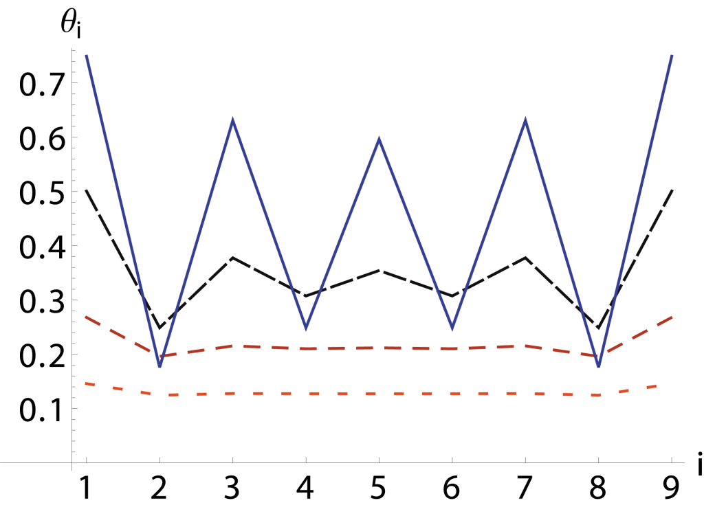
 , and
, and  , then
  nodes, where active nodes block their immediate neighbours. Define
  as a constant and
  as the number of neighbours of node
  , and
, and  voor
voor  , we see that the outermost nodes are assigned a lower activation rate than the other nodes. This is intuitively clear, as it compensates for the high throughput of the outer nodes in the case all activation rates are the same.
 , containing all possible combinations of throughputs that can be achieved by selecting the right activation rates. This set of course depends on the structure of the interference graph, and can be interpreted as the range of the function
  introduced in
  . This range can be characterised as the interior of the convex hull of all possible independent sets of the interference graph.
 is a vector of the throughputs values we wish to achieve. We are now looking for the solution
  of the system of equations
 is to determine that
  to
to  ,
,  At the end of each interval, the activation intensities rates
  can be adapted. Let
  , and adapt modify this recursively as follows:
 is the empirical throughput in the
  -th interval. It can be shown that for the right choice of
  indeed converges to a solution
  such that
 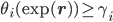 ,
,  [8]. This is a remarkable result, as the adjustment modification
  . To model the stochastic behaviour of the buffer contents, we introduce
  , where
  denotes the number of packets awaiting transmission or being transmitted at node
  of the various nodes is not influenced by the state of the buffers, and therefore maintains the equilibrium distribution
  is positive recurrent when
  for all nodes
  . The process
  is also Markovian, and behaves as a so-called quasi-birth–death process, for which the equilibrium distribution can be determined numerically by using so-called matrix geometric methods.
 are relatively high. In order to guarantee stability for such arrival rates, the throughputs
  also need to be relatively high, which in turn requires high activation rates
  . Such a regime is not only interesting theoretically but also relevant from a practical point of view. This is because a relatively high load can result in long delays and lower quality of the wireless service, while delays do not pose an essential problem in case of lower arrival rates.
 and activation intensities rates
  . We also focus specifically on an interference graph consisting of a square lattice of dimension
  , as illustrated in Figure 3.
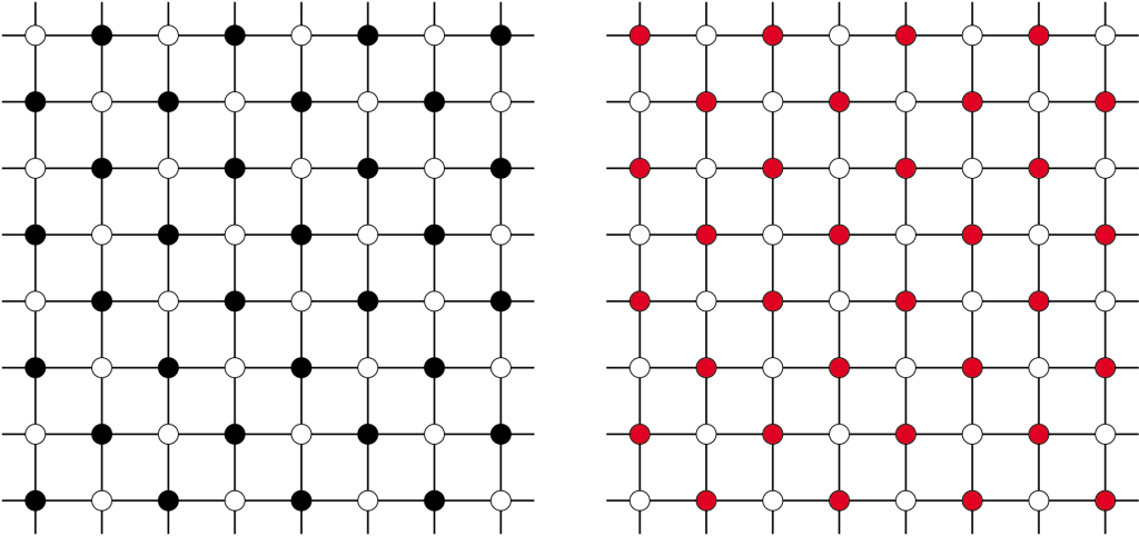
 , corresponding to the white and black fields of a chess-board, see Figure 3. For convenience refer to the maximum configurations and the corresponding nodes as 'even' or 'odd', respectively.
 for large values of
  equals
  or
or  , respectively, in the case of an open or periodic boundary. As a result, nodes that are not in the current active configuration will have no opportunity to transmit packets for a long time. For example, when the even configuration is active, packets arriving at the odd nodes will accumulate until at a certain time a transition occurs to the odd configuration, and the odd nodes will be given the opportunity to transmit a substantial number of packets in a row. The sequence of long periods of accumulation and transmission implies that the number of packets at an individual node evolves according to a saw tooth-like pattern, as illustrated in Figure 4. The amplitude of the saw tooth pattern is proportional to the associated timescale, and therefore roughly of the order O
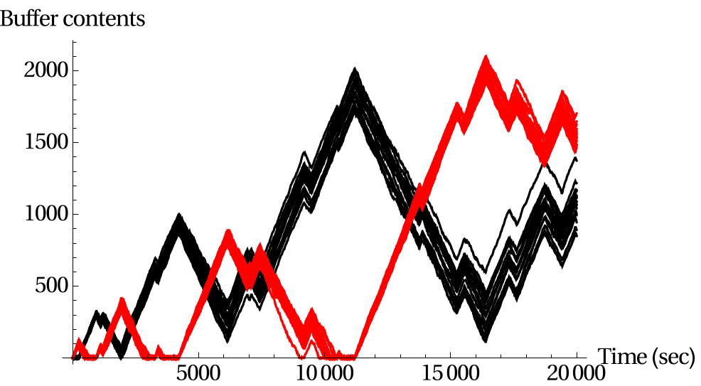
 and
and  are necessary conditions to ensure the stability of the system. We therefore conclude that the average number of packets contained in the buffer of an individual node is at least of the order of O
 when the arrival rate
  approaches the critical value
  [16]. Because of Little's Law, the average delay of a packet has the same order of magnitude. It is important to compare this scaling with the usual situation in conventional queueing systems where the average delay should be of the order of O
 . See for example [5] for an introduction to queueing theory. In other words, the slow transitions between the rigid maximum configurations have a strongly negative effect on the scaling of the number of packets and the delay, which furthermore gets worse with the size of the network as reflected by the exponent
  is not only determined by the activation process
  nodes and interference between nodes
  ,
,  ,
,  , and
, and  for the case when the buffers of all four nodes would be in a saturated condition. As a result, instability can occur at node
  is only slightly lower than the value
  of the number of packagespackets
  , where
  is a typically decreasing function and
  . For these model variations the Markovian character of the process
  , it is possible to determine the equilibrium distribution of the number of packets for several special choices of the functions
  and
and  [2]. The ratio of the functions
  increases super-linearly, linearly or sub-linearly with q. Because of Little's Law, the same three-way split occurs in the growth behaviour of the magnitude of the delay of the packets.
 nodes, the equilibrium condition of
  and
and  .. In the light of this observation it is even more remarkable that very explicit stability conditions have actually been identified, even though the proofs are very advanced. For a broad class of