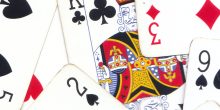
Four friends, Mark, Richa, Peter and Tom, play cards every evening. Peter is a probabilist while the other three work in algebra. On one evening they become bored of riffle shuffling.
Mark: Ah! I am so bored of riffle shuffling the decks. We don't even know why the deck is shuffled after riffle shuffling.
Richa: But everybody uses this and I heard Diaconis and Bayer showed that seven times riffle shuffling guarantees randomness of the deck.
Tom: Let's try some new shuffling idea today. Do you have any idea, Peter?
Peter: Actually, I know how riffle shuffle guarantees the randomness through the mixing time of a random walk on networks. In fact, we use riffle shuffle as it is the fastest shuffling method known until now. But if you want something new, I know another way of shuffling.
Mark, excitedly: Yeah, tell us about a new method please! I am keen to know!
Peter: Okay! I will tell you, but it may feel lengthy because it takes time whereas riffle shuffle takes only time. So, you need to be patient to apply this!
Mark: That's okay! Tell us!
The others agree by nodding their heads.
Peter: First take the deck and look at the bottom card. Remember it.
Then pick up the top card and put it anywhere between other cards uniformly at random. This means each position, or gap, is chosen with probability , as there are places to put the top card. Note that one of the options is to keep the top card where it is. This happens with probability . But if this happens, the next step is to move the top card again, until you do move it somewhere else. Keep doing this until the original bottom card comes to top and your deck will be shuffled. In other words, every permutation is (approximately) equally likely at the end of the shuffle.
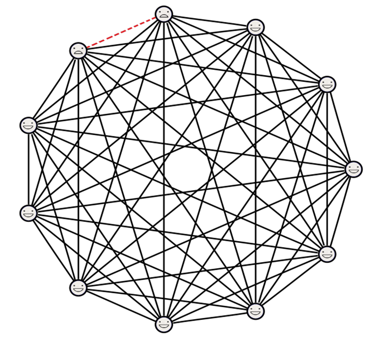
An animation illustrating Peter's proposed method of shuffling cards. The red card is the original bottom card. It shows the first three moves, but the shuffle is not yet complete.
Tom: Why so? Why is the deck then shuffled?
Peter: Be patient!
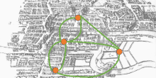
We can think of this method as a random walk on graph , where vertex set is , which are all possible permutations of . From any vertex (permutation) to another vertex , there is an edge if is obtained from in one step. From each permutation , the top card can be replaced to any of the possible gaps below. This implies that, from , we can reach any of those new permutations. Hence the degree of each vertex is and each edge-weight is .
This random walk has three important properties. First, there are finitely many permutations, so the number of vertices (or number of states) is finite. Second, you can reach any state from any other state in a number of steps. Consequenly, we say that the random walk is irreducible. Lastly, from any permutation we can reach that same permutation in one step with positive probability (in which case, the top card is placed in the 1st possible gap). It follows that the random walk is aperiodic.
So the random walk is irreducible, aperiodic and finite. The Fundamental Theorem of Markov Chains tells us that after enough steps, your starting permutation essentially does not matter any more. The state you will be in is irrespective of your starting vertex, but is still random. In mathematical terms, we know the step transition probability converges to it's stationary distribution for sufficiently large time . The most important question is: "is every permutation equally likely in the limit?" Or are some permutations more likely than others after the shuffle? The stationary distribution answers this question.
Calculating the stationary distribution is not that difficult. It turns out to be uniform over all permutations. This is exactly what you want for a card shuffle.
Peter grabs a napkin and writes down the calculation.
"The stationary distribution is given by "
Peter: This convergence is 'sufficient' when the walk reaches its mixing time. Thus we say this deck is uniform after mixing time is attained.
Richa: But how do we know that the random walk has reached mixing time after the shuffle?
Peter: That's an interesting question! Remember, I told you that we will stop when the original bottom most card comes to top. Think about this! When can this happen?
Mark: You said that we repeatedly place the top card to a random position under it. So, it means the original bottom card comes to top, when all other cards have been selected at least once and moved down.
Peter: Exactly! And we consider that permutation (when the bottom card is now on top) as a halting state. We then consider the optimal strong stationary time. Essentially, it can be shown that before reaching the halting state, the mixing is done with high probability.
Tom: Amazing! Great explanation. Can you tell how exactly you derived stationary distribution as ?
Peter: Do you guys know about detailed balance equation?
Mark: Yeah! For a Markov chain with transition probability and stationary distribution , detailed balance means and this happens when the Markov chain is reversible!
Peter: You are right! So, the transition matrix is…
Richa, interrupting Peter: So, from any permutation we are able to reach those of the permutations obtained by placing the top card in any of the gaps. Thus, the transition matrix is
\begin{equation*}P(\sigma, \tau) = \begin{cases} \frac{1}{\deg(\sigma)} = \frac{1}{n} \quad &\text{if $\tau$ is reached in one step from} \, \sigma \\ 0 \quad &\text{otherwise} \end{cases},\end{equation*} irrespective of states, right?
Peter: Correct! Now, the column sum of the transition matrix is . This is because every permutation can be reached in one step from exactly permutations, each with probability .
Combining and gives as an stationary distribution. And irreducibility along-with finiteness guarantees this as the unique stationary distribution.
Tom: Ah! Very interesting.
Peter: Now for any details about this mixing time and for the bounds, you can go through this book on Mixing Times by Levin-Peres-Wilmer.
Tom: Very cool! I never thought of using random walks and Markov Chain theory to analyze card shuffling. Does this also work for riffle shuffle?
An animation illustrating riffle shuffle, also seen in the cover photo.
Peter: Certainly! But it's more complicated, so I'll need some pieces of paper. Are you interested? Then I'll go get some.
Tom: Please! Riffle shuffle never gets old to me. I'd love to know why it works so well!
Peter: I'll be right back!
Part 2 about riffle shuffle will be published soon. Swastika Dey studies at the Indian Statistical Institute. She approached The Network Pages about writing this article. The animations were created by the Network Pages using Manim. The cover photo was taken from here.
Did you know that if you divide a pack of cards into 13 piles of 4 cards, then you can always pick one card from each of the 13 piles so that there is exactly one card with each rank? There is some beautiful math behind this puzzle.
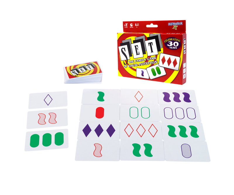
Most people are familiar with the game Set. A bunch of cards are laid out, and players race to spot a triple where each feature is either all the same or all different. What happens when we consider an expansion of this game?
Have you ever found yourself less popular when compared to your friends? Interestingly, in any group of individuals, on average, people have fewer friends than their friends do, or at the very most, an equal number. Not more!
 time whereas riffle shuffle takes only
  time. So, you need to be patient to apply this!
 , as there are
  places to put the top card. Note that one of the options is to keep the top card where it is. This happens with probability
  . But if this happens, the next step is to move the top card again, until you do move it somewhere else. Keep doing this until the original bottom card comes to top and your deck will be shuffled. In other words, every permutation is (approximately) equally likely at the end of the shuffle.
 , where vertex set
  is
is  , which are all possible permutations of
  . From any vertex (permutation)
  to another vertex
  , there is an edge
  if
if  .
. step transition probability converges to it's stationary distribution for sufficiently large time
  . The most important question is: "is every permutation equally likely in the limit?" Or are some permutations more likely than others after the shuffle? The stationary distribution answers this question.
 "
" ?
? and stationary distribution
  , detailed balance means
  and this happens when the Markov chain is reversible!
 gives
gives  as an stationary distribution. And irreducibility along-with finiteness guarantees this as the unique stationary distribution.