Have you ever wondered what mathematicians mean when they talk about mathematical models of real-life phenomena? And what can such a model tell us about the network-phenomenon we are studying? In this article we present a method used by various scientists when they want to understand how real-world networks work. This method is inspired from statistical physics, the physics of small particles!
Transportation networks, communication networks and social networks form the backbone of modern society. In recent years there has been a growing fascination with the complex connectedness such networks provide.
This connectedness manifests itself in many ways: in the rapid growth of Internet and the World-Wide Web, in the ease with which global communication takes place, in the speed at which news and information travel around the world, and in the fast spread of an epidemic or a financial crisis. These phenomena involve networks, incentives, and the aggregate behaviour of groups of people. They are based on the links that connect people and their decisions, with global consequences.
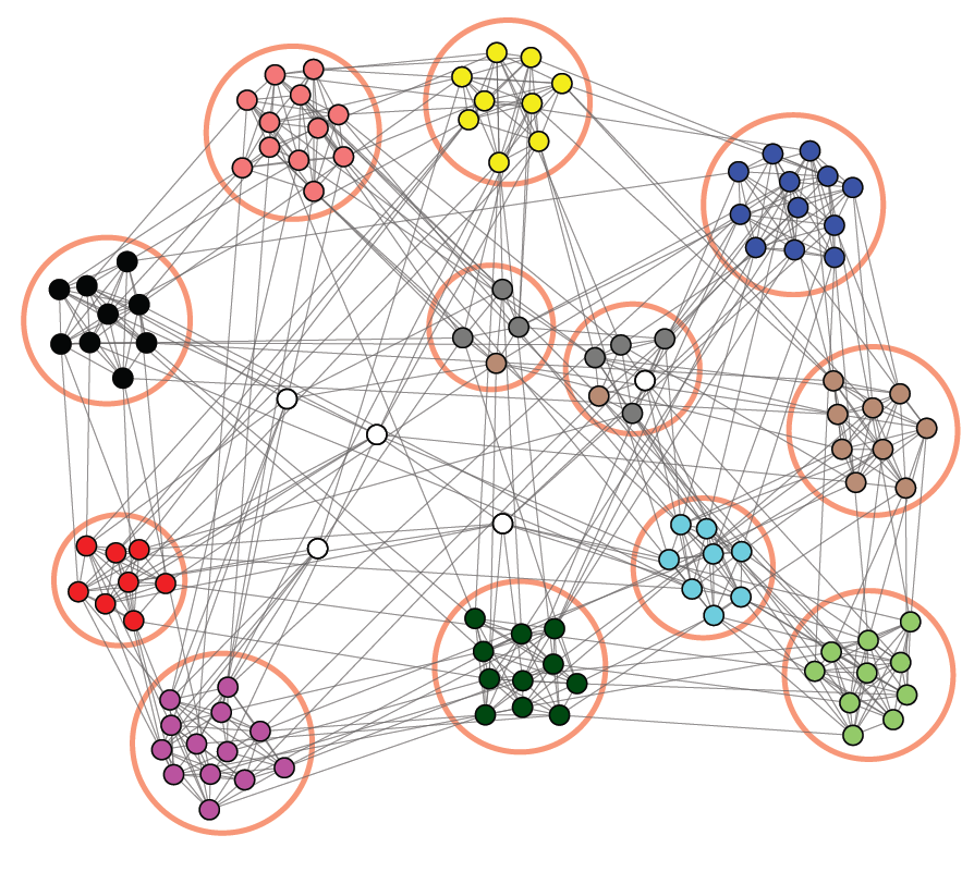
Example of real life network: the LinkedIn network of Olivier Duquesne
A network can be viewed as a graph. The vertices in the graph represent the nodes of the network, the edges connecting the vertices represent the links between the nodes. Neurons in the brain are connected by synapses, proteins inside the cell by physical contacts, people within social groups by common interests, countries of the world by economic relationships and financial markets, companies by trade, and computers in the Internet by cables transferring data. Despite the very different origin and nature of these links, all systems share an underlying networked structure representing their large-scale organisation. This organisation in turn leads to self-organisation, and other emergent properties, which can only be understood by analysing the overall architecture of the system rather than its constituents elements alone.
Dutch railway network and the degree histogram. The degree of a station corresponds to the number of other stations that are directly connected railway to the station. [3]
Most complex networks display non-trivial geometric features, with patterns of connection that are neither purely regular nor purely random. The challenge is to understand the effect such features have on the "performance" of the network, via the study of models that allow for computation, prediction and control.
From interacting particle systems to complex networks
In a preceding article we explained the importance of ensembles for the study of interacting particle systems with given constraints (such as total energy and/or total number of particles). We now take a look at ensembles for complex networks.
Just like the traditional ensembles in statistical physics, ensembles of random graphs are constructed from a set of given constraints. Such constraints represent the structural properties we would like to impose on the graph to make it allowable. For instance, we may require that the graph has a specified total number of links. As for the traditional ensembles, this constraint can be either hard or soft, which leads to two different ensembles ("microcanonical" or "canonical") for the same constraint. In general, the constraint can refer to a more complicated structural property, e.g. there can be multiple constraints. Ensembles of random graphs with constraints are used in a variety of different applications. Two examples, which we briefly describe below, are pattern detection and network reconstruction.
Pattern detection. This is the search for non-trivial structural properties in a real-world network, through comparison with a random graph model that captures some of the observed geometric properties (treated as constraints). For instance, we may wonder whether the number of triangles that is observed in a real-world network is unusually large or unusually small, given the total number of links in the network. This would lead us to use a null model, defined as an ensemble of graphs with the same number of links as the real-world network. The observed number of triangles can then be compared with the expected number of triangles in the associated random ensemble. If the two numbers are consistent with each other, within statistical bounds, then we can conclude that the empirical abundance of triangles is compatible with the null hypothesis that the structure of the network is captured by the null model.
However, if the two numbers are not consistent with each other, then triangles might be a "pattern" for the network and therefore require a more complicated explanation than that encoded in the chosen constraint. Most real-world social networks indeed feature a surprisingly high clustering coefficient, defined as the fraction of realised triangles in the network. This pattern is therefore a topological signature of the tendency of people in social networks to form more triangles than is expected by chance on the basis of the overall density of links in the network. Another empirically widespread pattern is the presence of so-called communities in real-world networks, i.e., groups of nodes that are internally more densely connected than expected by chance under a suitable null model. Again, the latter is defined as an ensemble of random graphs with given properties. Identifying communities is important in order to resolve the modular structure of real-world networks. In turn, this modular structure helps to decompose the description of very large networks into that of smaller sub-networks.
Network reconstruction. This employs purely local geometric information (again treated as constraints) to infer non-local properties of a real-world network, whenever the structure of the latter is not known completely (for instance, because of confidentiality or privacy issues). An important example is provided by interbank networks, which are one of the key channels through which financial distress can propagate, possibly leading to large-scale banking crises. In the wake of the 2008 crisis, it has become clear that the structure of real-world interbank networks crucially determines whether and how fast financial defaults can cascade throughout the system. Bank regulators and policy makers should in principle have access to the full network in order to reliably supervise the banking system. Unfortunately, the links of the network (which represent the debt/credit relationships among banks) are protected by confidentiality issues and are often unobservable. It is therefore necessary to reconstruct the structure of the network probabilistically, starting from the partial information that is available. Since the total exposure of each bank to all other banks is typically known (this information is typically public), one way to infer the hidden structure of the network is via the construction of an ensemble of random graphs where the constraints are the total exposures of all the banks. This graph ensemble is defined by multiple constraints (one constraint per node). Unlike the other examples we mentioned so far, the number of constraints increases as the number of nodes increases.
Consequences. In the above two applications, the constrained ensemble can be realised either micro-canonically or canonically, and the choice is often based only on mathematical or numerical convenience. However, this freedom of choice is justified only when the ensembles are asymptotically equivalent. If ensemble equivalence breaks down, then the choice of ensemble should be principled, i.e., dictated by an independent theoretical criterion that indicates a priori which ensemble is the appropriate one. For instance, when the constraints are hard in the real-world network, but are treated as soft in the chosen ensemble, this leads to an unnecessary level of uncertainty in the probabilistic microscopic description, making the latter more noisy than needed. However, in the applications mentioned above, we are usually in the opposite situation, where the empirical constraints are necessarily subject to measurement errors (for instance, there can be mistakes or accounting errors in the reported exposure of a bank). The empirical value of each constraint should therefore be treated as the most likely value for an underlying uncertain quantity, and so each constraint should be treated as soft. Treating an intrinsically soft constraint as a hard constraint means propagating the measurement error to the entire ensemble and introducing a strong bias: configurations where the constraint has a value that is only slightly different from the measured value would be given zero probability, whereas these configurations are expected to have a probability that is only slightly smaller than the probability of the configurations that match the measured value of the constraint precisely.
Breaking of ensemble equivalence for complex networks
In order to study the breaking of ensemble equivalence for complex networks, we replace particles by nodes and interactions between particles by links between nodes. Thus, our system is composed of nodes that may be connected to each other via possible links. Each link can be either present or absent. Two examples of constraints are:
Fix the total number of links to be i.e., a fraction of possible links are present.
Fix a degree sequence to be , i.e., the degree of node is .
We are interested in what happens in the limit as subject to these constraints .
Relative entropy
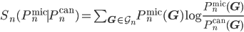
In order to study breaking of ensemble equivalence, we use the notion of relative entropy per node. Let be the set of all simple graphs with nodes (no self-loops and no multiple edges). Let and denote the micro-canonical, respectively, canonical probability distribution on corresponding to a given constraint. We say that and are equivalent when their entropy, defined by
satisfies
As shown in references [1] and [2], for the two examples of constraints mentioned above:
ensemble equivalence holds,
ensemble equivalence is broken.
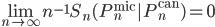
Many other examples, including graphs with a community structure like in the figure below, have been studied in reference [1] and [2]. These show that, as soon as the number of constraints is of order of the size of the network, the equivalence between the two ensembles is broken.
Network with communities (snap.stanford.edu).
References
[1] D. Garlaschelli, F. den Hollander, and A. Roccaverde, Mathematics Archive, 1603.08759.
[2] T. Squartini, J. de Mol, F. den Hollander and D. Garlaschelli, Physical Review Letters, volume 115, page 268701 (2015).
[3] Picture of the rail-network by Dennistw [CC BY-SA 4.0 (http://creativecommons.org/licenses/by-sa/4.0)], via Wikimedia Commons
One of the main building blocks of modern AI-tools are artificial neural networks, abstract models inspired by the structure and functions of biological neural networks which enable machines to "learn". In this article, I will discuss some thoughts on this topic.
During our teenage years, everything changes. It’s no surprise that our brain does too. But how do we make sense of this transformation? Is there a way to quantify it? Networks might just be the answer.
We want our guts to be filled with a diverse range of mutually beneficial and competitive interactions, a perfect blend of friends, frenemies, and enemies to keep our guts active and body on its toes. Read how networks can help understand these interactions!
After more than ten incredible years, the NETWORKS programme will officially conclude at the end of 2025. In light of this approaching milestone, the final NETWORKS conference & reunion took place.
In November 2024, the Kick-Off meeting for BeyondTheEdge: Higher-Order Networks and Dynamics took place at Vrije Universiteit (VU) Amsterdam. The event marked the official start of the project, read an interview with Christian Bick, Principal Investigator and Project Coordinator of BeyondtheEdge.


 nodes that may be connected to each other via
  possible links. Each link can be either present or absent. Two examples of constraints are:
 i.e., a fraction
  of possible links are present.
 , i.e., the degree of node
  is
is  .
. subject to these constraints .
 be the set of all simple graphs with
  and
and  denote the micro-canonical, respectively, canonical probability distribution on