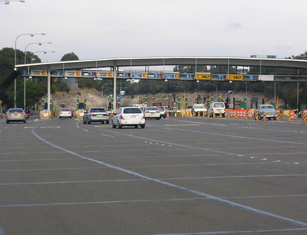
In a preceding article we have used a simple model to demonstrate how selfish behavior can create additional congestion. One way to mitigate the consequences of selfish behavior, is by introducing tolls (or taxes) on certain parts of the road network. This is also known as road pricing, and such a system was first successfully implemented in Singapore (click here for more info).
The idea is that drivers will not only choose their route based on the travel time along a path through the network, but they will also take into account the toll or tax they have to pay on that path. This toll may vary along the day (think of higher tolls during rush hour) or can depend on the amount of traffic congestion on certain parts of the network. The goal is to choose the tolls in such a way so that the traffic spreads out nicely over all paths, leading to an efficient (or even optimal) usage of the network.
In the remainder of this article, we will see how tolls can be used in order to improve the inefficient network usage in Pigou's example from the previous article. The Pigou network is given below. The latency functions on the arcs, describing how long it takes to travel between the two points, are and where is the amount of traffic on arc . One unit of flow has to be divided over the two arcs.
In the selfish equilibrium , all flow is sent over the first arc, that is, . In the social optimum , the flow is split among the two arcs, that is, (see the previous article for details).
We now explain how the tolls are modeled. On every arc , we introduce a non-negative (constant) representing the toll. The new objective of the drivers is to minimize a combination of latency and toll. At first this might seem somewhat strange, since is interpreted in terms of time, and in terms of money. We assume that drivers 'transform' the toll into time, e.g., 10 euros might correspond to 30 minutes of travel time. This transformation is modeled by the (sensitivity) parameter . The new objective of the drivers is now to minimize the combined cost . In the example above, we have (if we measure time in minutes and money in euros). Of course, different drivers might make different transformations, but here we assume they all do this in a similar way, i.e., we say the drivers are homogeneous. If different drivers make different transformations, we call them heterogeneous. This can be represented in the combined cost by introducing parameters that represent the transformation factor of the -th class of drivers, i.e., the combined cost then becomes for the drivers in class .
Another important modeling assumption is that we assume that (for example) a government is not interested in the profits they make from this toll system, that is, their (quantitative) measure for system performance is still the average travel time. This can be justified in many ways. E.g., it might be the case that the tolls are needed to pay for the implementation of the toll systems. Or, in case the average travel time measure is used as an indication for the emission of green house gasses, the obtained tolls do not play a role, since these do not (directly) decrease the emission of green house gasses.
The main question is now: How should the tolls be chosen in order to decrease the average travel time? Or even better, to achieve the smallest possible average travel time. We call the traffic flow creating the smallest average travel time the social optimum. For Pigou's example, we have seen that the average travel time is minimized for the social optimum , meaning that half of the traffic takes the upper road and the other half takes the lower road. This flow is not an equilibrium with respect to the latencies as and . So, how should we choose the tolls such that the combined costs are at equilibrium, meaning that
Exercise 4: How to choose the tolls and , such that the both roads are used according to the social optimum ? Consider that the drivers base there decision on the combined costs, and for simplicity, assume that .
How many of combinations of and can you find? Which combination minimizes the sum of the tolls?
Solution to Exercise 4: The drivers will split over the two possible road such that the combined cost of the road are equal, that is, . We would like to choose the tolls such that in this case. We find or equivalent . Since there are no further restrictions on the tolls (apart form the fact that they should be non-negative), we see that there is an infinite amount of possible combinations for and . A solution minimizing the sum of the tolls is given by and .
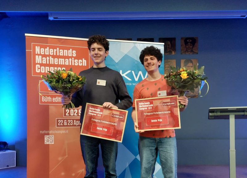
Getting to class on time isn't hard, if you leave on time and know the fastest route. But what’s the fastest route when the hallways are crowded? For their final high school project, Dylan and Tobias worked on finding the most efficient ways to navigate school during peak hours.
Elisabeth already has an idea in mind: she would like to find the fastest possible route that goes to each address exactly once before finally returning to the station. This task is a well-known mathematical problem, namely the Traveling Salesman Problem (TSP)! How can she solve it?
During our teenage years, everything changes. It’s no surprise that our brain does too. But how do we make sense of this transformation? Is there a way to quantify it? Networks might just be the answer.
One of the main building blocks of modern AI-tools are artificial neural networks, abstract models inspired by the structure and functions of biological neural networks which enable machines to "learn". In this article, I will discuss some thoughts on this topic.
If, after reading the title, your immediate response is to shout "1/6-th", then you have correctly answered the question. Well done! However, in this article we will focus on the meaning of this question. What exactly is this "chance" of which you've just exclaimed it equals 1/6-th?
 and
and  where
where  is the amount of traffic on arc
  . One unit of flow has to be divided over the two arcs.
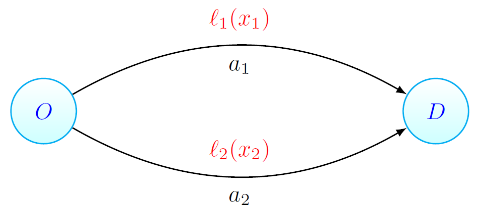
 , all flow is sent over the first arc, that is,
 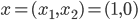 . In the social optimum
  , the flow is split among the two arcs, that is,
 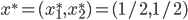 (see the previous article for details).
 , we introduce a non-negative (constant)
  representing the toll. The new objective of the drivers is to minimize a combination of latency and toll. At first this might seem somewhat strange, since
  is interpreted in terms of time, and
  . The new objective of the drivers is now to minimize the combined cost
  . In the example above, we have
  (if we measure time in minutes and money in euros). Of course, different drivers might make different transformations, but here we assume they all do this in a similar way, i.e., we say the drivers are homogeneous. If different drivers make different transformations, we call them heterogeneous. This can be represented in the combined cost by introducing parameters
  that represent the transformation factor of the
  -th class of drivers, i.e., the combined cost then becomes
  for the drivers in class
  and
and  . So, how should we choose the tolls
  such that the combined costs
  are at equilibrium, meaning that
 and
and  , such that the both roads are used according to the social optimum
  .
.