Below are two photos of Itteren, a town in the south of the Netherlands. The first one shows the town as it looks normally. The second picture shows, well, quite an extreme: a flood. In 1995, this flood led to the evacuation of 250 000 people and a million animals. This was one of a handful of heavy floods in the 90's, so the Dutch regional water authorities (water boards, or "waterschappen" in Dutch) were tasked with calculating how often an area overflows. Based on these calculations, the Dutch government took better protective measures against floods. How do these calculations work?
Figure 1 and 2: The town of Itteren, Limburg, in 2016 (left; Van de Biezen, 2016) and 1995 (right; Rijkswaterstaat, n.d.)
These calculations are called flood frequency analyses. The objective: calculate if an area does not overflow "too often". Although floods are rarely desirable, they may be acceptable on occasion. For example, preventing a flood might be more expensive than dealing with the consequences if water reaches your house only once every hundred years. In this case, you may choose to let the flood happen, whenever that may be, and repair the damage when it does. Flood frequency analyses are done using one of two statistical methods; the "timeseries method" or the "stochastic method". Different water boards use different methods, the division being roughly 50/50. We don’t actually know, however, if these methods lead to different results. Spoiler alert: they do!
I had the opportunity to research both methods for Waternet, the company that works on behalf of water board Amstel, Gooi en Vecht. They use the timeseries method for the flood frequency analyses, but were also interested in implementing the stochastic method as there may be advantages to using one method over the other.
The objective
First, we must ask ourselves: how often is 'too often'? The Dutch provinces have decided on an acceptable return period , measured in years, for each type of area. According to the provinces, the type of area is allowed to flood once every years. For instance, the provincial bylaws note that a house is allowed to flood once every hundred years (). By law, the water boards have to take measures making sure that water does not reach houses more often than that. Another example is farmland, which is allowed to flood only once every twenty-five years.
The water authorities use statistics and hydrological software to calculate the water level that corresponds to return period . What does this mean exactly? Say, we want to do a flood frequency analysis for farmland. That means that, given the provincial bylaws, we look for the water level corresponding to . If the water level corresponding to is higher than the level of the farmland, Waternet has to take measures to ensure this area overflows less often than once every tenty-five years. The number can take every value above zero, but common values (extracted from the bylaws) are ten, twenty-five, fifty and a hundred years.
A digital tool for mapping floods
The hydrological software D-Hydro can be used for both the stochastic and timeseries method. Using D-Hydro it is possible to map different areas into systems of canals, rivers, pumps, bridges and more. Figure 3 shows how this looks.
Figure 3: The Noordse Buurt and Westveense polder as simulated in D-Hydro.
D-Hydro can be given various input parameters and calculates water levels based on those inputs. Both the stochastic and timeseries method use the water levels calculated by D-Hydro. The difference between the methods is the input and the way its output is used to calculate how often an area floods.
The timeseries method
Let's start by looking at the timeseries method. In De Bilt the Royal Dutch Meteorological Institute (KNMI) records the amount of precipitation. These records are available as a dataset with hourly measurements, going back over a hundred years. These "rainfall events" are the input for D-Hydro, which then calculates the water levels over time.
After entering the rainfall events into D-Hydro and calculating the water levels, we select the highest water level per year. So, over the total years, we obtain with different maximum water levels. We denote these by . We call the maximum water level in a year , which is a random variable. The water levels are realizations of .
Ideally, we want to know the distribution of as it holds all kinds of relevant information. Extreme Value Statistics (EVS) can help with this. EVS has important results on the the maximum values of random variables, namely that the distribution of the maximum over many independent draws always converges to a specific probability distribution. If we assume that necessary conditions for EVS are met, we can use it to gain insight into the yearly water peak, in this case . EVS is a commonly used method for estimating flood events and it has many other applications.
Some extra clarification for the interested reader: As described, the first step is to take the different water levels, which are yearly maxima. We sort these water levels in a non-rising order. Denote by the rank of in the sorting. For example, if would be the highest water level recorded over all the years, . The second highest water level would get rank and so on. Next, we define
\begin{equation}
P_k = \frac{m_k}{n+1}, \quad, \text{for $k=1,\dots,n$}.
\end{equation}
Here, is an approximation of the probability of exceedance of . So,
\begin{equation}
P_k \approx \mathbb{P}(W > w_k),
\end{equation}
meaning the chance that a random maximum water level in an arbitrary year is higher than . Extreme value statistics tells us that, under certain assumptions, it holds that
\begin{equation}
1 - P_k = \mathbb{P}(W \leq w_k) \approx -e^{-e^{-(w_k-b)/a}},
\end{equation}
for some constants and . This distribution is known as the Gumble distribution. From this we can deduce that
\begin{equation}
w_k \approx a\big(-\ln(-\ln(1-P_k))\big) + b.
\end{equation}
If we define
\begin{equation}
Y_k = -\ln(-\ln(1-P_k)),
\end{equation}
we see that , so it follows a linear trend.
In practice, we want to compute the water level for a given return period . We define and calculate analogously to before, so
\begin{equation} Y_\tau = -\ln(1/\tau), \end{equation} and compute
To use this result, however, we need to know and . A common approach is to use linear regression. In consultation with Waternet, a different approach was chosen: to do linear interpolation between the two surrounding datapoints.
Essentially, we plot the datapoints with on the x-axis and on the y-axis. We connect the datapoints by straight line segments.
Precisely, to get , we compute
\begin{equation}
\hat{w}_\tau = w_L+\frac{Y_\tau-Y_L}{Y_R-Y_L}(w_R,w_L), \quad \tau>0,
\end{equation}
where are are values closest to ( on the left, on the right hand side) and and the corresponding water levels ( is left, on the right hand side). Our is an estimator of .
To give a more concrete, theoretical example: Say, we have a five-year series of rainfall events. From this five-year series, we get five different yearly maximums. See the table below for an example of these maximums, with the calculated , and .
Input
Date
Water level (m+NAP)
Rank
Probability
Z-Score
1
2006
2
2
2007
1
3
2008
5
4
2009
4
5
2010
3
We want to estimate the water level for a return period of . This gives us a of , which gives of .
The closest ’s are on the right hand side and on the left hand side. Filling this in, for our estimator , gives: \begin{equation} \begin{split}\hat{w}_{\tau=5}&=-3.50+\frac{(1.609-0.903)}{(1.702-0.903)}(-3.41+3.50)\\&=-3.42.\end{split}\end{equation}
To conclude, using this theoretical dataset, we estimate the water level to reach every five years.
A note on assumptions: Here we assume that follows a Gumble distribution. Extreme Value Statistics tells us this is the case if certain assumptions are met. Let us look at some of those assumptions. The Fisher-Tippett-Gnedenko theorem or its more general counterparts gives us an asymptotic distribution of if the observations that induce (in this case the measurements of water levels) are independent. This is not necessarily the case, as the water level on a given day may be correlated with the water level on surrounding days. More recent work shows that the asymptotic behaviour still holds if the dependence is "weak enough". The theorem also gives other possible asymptotic distributions, other than Gumble. If water levels are heavy-tailed, for instance, another asymptotic distribution comes into play. The validity of the assumptions underlying this method are an important and interesting topic of discussion, but outside the scope of this article.
The stochastic method
With the stochastic method, we say that a whole plethora of explanatory variables can cause extremely high water levels. For example, if the water level in a river is extremely high, just a bit of rain can cause a flood. The same goes for if a pump fails: if water cannot be pumped out of a polder, canals might overflow, even without rain.
These (continuous) explanatory variables are discretized in different classes, after which every class gets a representative value. The goal being that every possible situation that might happen, gets simulated in D-Hydro. Every class gets allocated a probability, based on historical data from a case study area.
The advantage of this method is that we don’t just look at rainfall events to predict floods, but also look at other contributing factors. With enough historical data, we can add almost any contributing variable, like how high the groundwater level is, the water levels in neighboring rivers and lakes, and lastly also if certain pumping stations fail.
Let be the explanatory variables. The probability that takes the value , meaning it is in the -th class, is denoted by by These are approximated using historical data.
The probability that an input vector occurs is approximated by multiplying the probabilities that variable falls in class .
In other words, we assume that the random variables are independent.
For every possible input vector , we perform a simulation in D-Hydro, which gives the corresponding water level . Using these, we can compute the probability of exceeding a given water level as follows:
Within this method we also use interpolation to estimate . Here we don’t interpolate based on a reduced variable (like we did with the timeseries method), but on our previously calculated and . So
To give a more concrete, theoretical example: Say we have two theoretical variables and The probability of it being summer or winter is equal, 0.5, for either both. However, the chance of less than 20 millimeters of precipitation is 0.7, and more then 20 millimeters is 0.3. This gives us the following table:
Input vector
(summer,≤20)
0.35
−3.62
(summer,>20)
0.15
−3.55
(winter,≤20)
0.35
−3.65
(winter,>20)
0.15
−3.59
To calculate our , we simply add the calculated probabilities of the water levels that are higher then the we seek. So, for , the water levels that are higher or equal, are itself, and . Which gives
Usually we have a couple of hundreds inputs, as opposed to only a few in this theoretical example. So we cannot really estimate our 's in this example. However, it works in the same way our timeseries method works.
What does the result look like?
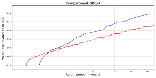
Both methods ideally lead to the same result, which is a graph with on the logarithmical x-axis our return periods (the we are after), and on the y-axis the water level (the we seek). In Figure 4, the result is shown for one area (compartment OP-1-A) in the Noordse Buurt and Westveense polder, our case study region. In every of the thirty compartments in our case study, the timeseries method lead to higher predicted water level compared to the stochastic method. The average difference over all compartments was 4 to 9 centimeters, with ranging from 25 to a 100 years. The maximum difference was over 28 centimeters.
Figure 4: Results of the stochastic method (red) and the time series method (blue) for compartment OP-1-A in the Noordse Buurt and Westveense polder.
Now knowing that these two methods lead to varying results, it is interesting to know why we get these varying results. In turn, this could help the water boards make more informed decisions in what measures to take and when. During my research at Waternet, I investigated multiple explanations for these differences, about which I write in my thesis Schatten van wateroverlast, een vergelijking tussen statistiek vóóraf en statistiek áchteraf in de Noordse Buurt en Westveense polder (De Beus, 2025). As you can tell, it is written in Dutch.
My experience at Waternet
As an applied mathematician, I never imagined myself suddenly doing my thesis at a company which regulates and takes care of our water supply and systems. It is a fun example of how mathematics is almost everywhere! I found myself in a team of hydrologists, which is a whole other area of expertise, I thought. However, all models they use (including D-Hydro) were based on, as you might guess, mathematical models and formulas. Furthermore, these two methods I researched are largely mathematical problems. The hydrological part is mapping the water system in D-Hydro, and knowing how to take correct measures.
The models I implemented were immediately used for other case study areas. Through my research I hoped to give better insight on how and when to implement which method. Most importantly, I wanted to shed light on some of their drawbacks and when these drawbacks influence the results.
Cover photo taken from Orange County Register, June 19th, 2008
As soon as plastic waste ends up in water, it becomes increasingly difficult to clean up. That’s why it’s important to capture the waste closer to its source, in these canals and rivers. How can mathematical models be used to help clean plastic waste from canals and rivers?
The gut microbiome works hard to keep you healthy. To understand it, we need to know how nutrients travel through the gut. This is where gut flow enters the story. How can we simulate gut flow with mathematics?
The scientific world would not be what it is today without normal distribution. It is the foundation of many statistical models for several good reasons. Most importantly, it appears commonly in nature. But this is only the tip of the iceberg.
Two weeks ago I had the pleasure to attend two events where prizes for outstanding research in mathematics were awarded, one of them was the CWI Best Thesis in Applied Math 2024. It was a great pleasure to be there, to chat with (most of) the candidates, and to learn what they have done during their bachelor and master thesis'.



 , measured in years, for each type of area. According to the provinces, the type of area is allowed to flood once every
  ). By law, the water boards have to take measures making sure that water does not reach houses more often than that. Another example is farmland, which is allowed to flood only once every twenty-five years.
 that corresponds to return period
  . If the water level corresponding to
  is higher than the level of the farmland, Waternet has to take measures to ensure this area overflows less often than once every tenty-five years. The number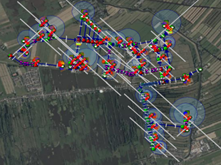
 total years, we obtain with
  . We call the maximum water level in a year
  , which is a random variable. The water levels
  are realizations of
  in a non-rising order. Denote by
  the rank of
  in the sorting. For example, if
  would be the highest water level recorded over all the years,
  . The second highest water level would get rank
  and so on. Next, we define
 is an approximation of the probability of exceedance of
  and
and  . This distribution is known as the Gumble distribution. From this we can deduce that
 , so it follows a linear trend.
 and calculate
  analogously to before, so
 on the x-axis and
  on the y-axis. We connect the datapoints by straight line segments.
 are are values closest to
  on the left,
  on the right hand side) and
  and
and  the corresponding water levels (
 is an estimator of
  .
. 


 . This gives us a
  of
of  , which gives
  .
. on the right hand side and
  on the left hand side. Filling this in, for our estimator
  every five years.
 be the explanatory variables. The probability that
  takes the value
  , meaning it is in the
  -th class, is denoted by by
  These are approximated using historical data.
 occurs is approximated by multiplying the probabilities that variable
  .
. are independent.
 . Using these, we can compute the probability of exceeding a given water level
  is the approximation of the chance that the water level exceeds level
  and
and  . So
. So and
and  The probability of it being summer or winter is equal, 0.5, for either both. However, the chance of less than 20 millimeters of precipitation is 0.7, and more then 20 millimeters is 0.3. This gives us the following table:
 , we simply add the calculated probabilities of the water levels that are higher then the
  , the water levels that are higher or equal, are
  itself,
  and
and  . Which gives