Congested road networks are a big problem in many countries. Building more roads is not always the best solution to solve this issue. One of the reasons for this is that drivers behave selfishly (trying to have the shortest possible travel time to get from work to home), which leads to inefficient usage of the road network as many drivers want to use the same parts of the network.
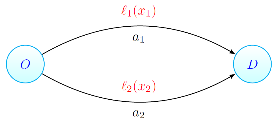
An example of this phenomenon, called Pigou's network, is given in this article. Tolling schemes are a way to enforce selfish drivers (equilibrium flow) adopt a driving behavior which decreases the average travel time of all drivers (social optimal flow)!
In the preceding article we showed how tolls (or taxes) can be used to mitigate the effects of selfish routing in Pigou's network. In particular, we computed tolls with the property that if players minimize a combined cost of latency and toll, the resulting equilibrium flow is precisely the socially optimal flow. This means that the network is being used efficiently. Do such tolls always exist? We only showed this for one pair of latency functions, but what about arbitrary latency functions? This question has been answered affirmative by Beckmann, McGuire and Winston already back in 1956. This was a couple of years after the introduction of Wardrop's routing model in 1952, which is a general description of the model we consider here. They showed that optimal tolls, to induce the socially optimal flow as equilibrium flow, always exist (under some mild assumptions on the latency functions)!
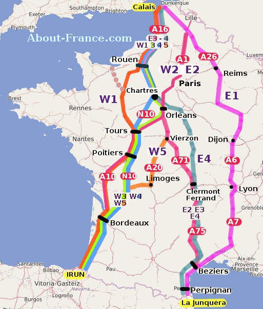
Figure 1: Toll maps in Ireland (Left panel) and France (Right panel, Photo from AboutFrance.com)
In this article we will describe how to set tolls in such a way that the socially optimal flow becomes an equilibrium flow. We do this for arbitrary latency functions that satisfy some basic assumptions. For simplicity, we focus on Pigou's network. Our goal is to give an intuitive argument for what these tolls should look like. The general result uses techniques from convex programming .
We first make some mild assumptions concerning the properties the latency functions and should have. As before, we assume that they are non-negative and increasing (to mimic the effect of congestion). Moreover, we also assume that both functions are differentiable.
Remember that the social cost of a flow is given by the average travel time in the network, which is We will call the social optimum as before. Suppose that there is a positive amount of flow on the upper road: . Since the flow is optimal, this means that if we would shift some small amount of flow from the upper to the lower road, then the social cost of the resulting flow can't be better than the cost of flow . An important concept here is the rate of change in social cost on a road, which is precisely the derivative of the term . Using the chain rule, we get that
where is the derivative of the function .
If we shift an amount of from the upper to the lower road, then the social cost decreases by approximately on the upper road, and increases by approximately on the lower road. This approximation is valid, since is very small. Because is a socially optimal flow, the increase of social cost on the lower road cannot be higher than the decrease of social cost on the upper road. Said differently, we must have . Using the expression for the derivative given above, this is the same as saying that
Now, let us think back of what it means to be an equilibrium flow under a tolling scheme. If we have tolls and on the roads, and there is a positive amount of flow on the upper road, then the equilibrium conditions tell us that the combined cost of latency and toll on the upper road must be smaller or equal than that of the lower road. Otherwise some small fraction of flow could switch to the lower road to get a better combined cost. Stated mathematically, if is an equilibrium for the tolls and , then we must have
Comparing the last two inequalities, it follows that if we set
then indeed the flow on the upper road cannot get a better combined cost by switching to the lower road. We can of course use completely analogue arguments if we would use the lower road as a starting point. This shows that the tolls given above indeed give the social optimum as equilibrium flow for the combined cost of latency and toll!
References
Beckmann, M., McGuire, C.B., Winston, C.B.,: Studies in the economics of transportation. Yale University Press, New Haven (1956)
J. G. Wardrop. Some theoretical aspects of road traffic research. Proceedings of the Institution of Civil Engineers, 1:325–378, 1952.
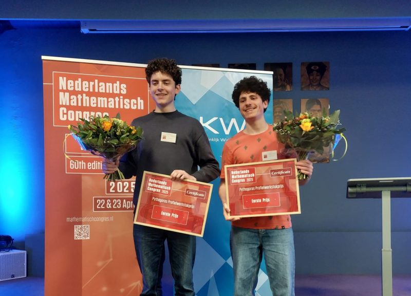
Getting to class on time isn't hard, if you leave on time and know the fastest route. But what’s the fastest route when the hallways are crowded? For their final high school project, Dylan and Tobias worked on finding the most efficient ways to navigate school during peak hours.
In October 2025 a masterclass on networks and algorithms will again be organised by the mathematics research program NETWORKS. Teachers and school students at the level of VWO 5-6 are welcome to join this two-day masterclass, no specific prior knowledge is needed, only enthousiasm about mathematics!
When we fight for limited common resources, our decisions will shape opponents’ responses and vice versa. What does mathematics have to say about such situations?
![[1]](https://www.networkpages.nl/wp-content/plugins/latex/cache/tex_35dba5d75538a9bbe0b4da4422759a0e.gif) already back in 1956. This was a couple of years after the introduction of Wardrop's routing model
already back in 1956. This was a couple of years after the introduction of Wardrop's routing model ![[2]](https://www.networkpages.nl/wp-content/plugins/latex/cache/tex_beb4dbf9af069aa2df7b147229965085.gif) in 1952, which is a general description of the model we consider here. They showed that optimal tolls, to induce the socially optimal flow as equilibrium flow, always exist (under some mild assumptions on the latency functions)!
in 1952, which is a general description of the model we consider here. They showed that optimal tolls, to induce the socially optimal flow as equilibrium flow, always exist (under some mild assumptions on the latency functions)!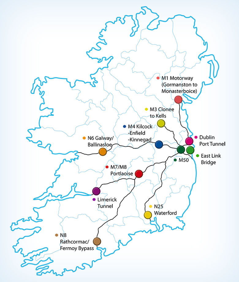
 and
and  should have. As before, we assume that they are non-negative and increasing (to mimic the effect of congestion). Moreover, we also assume that both functions are differentiable.
 is given by the average travel time in the network, which is
  We will call
  the social optimum as before. Suppose that there is a positive amount of flow on the upper road:
  . Since the flow
  from the upper to the lower road, then the social cost of the resulting flow can't be better than the cost of flow
  . Using the chain rule, we get that
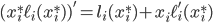
 is the derivative of the function
  .
. on the upper road, and increases by approximately
  on the lower road. This approximation is valid, since
 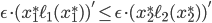 . Using the expression for the derivative given above, this is the same as saying that
 and
and  on the roads, and there is a positive amount of flow on the upper road, then the equilibrium conditions tell us that the combined cost of latency and toll on the upper road must be smaller or equal than that of the lower road. Otherwise some small fraction of flow could switch to the lower road to get a better combined cost. Stated mathematically, if
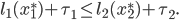
 given above indeed give the social optimum as equilibrium flow for the combined cost of latency and toll!